Generating publication quality figures
using R & ggplot2
Guangchuang Yu
Jul. 24, 2014
Why ?
- There are so many biologists use excel for graphing.
- It's easy to create a barplot in excel, but hard for boxplot.


Power
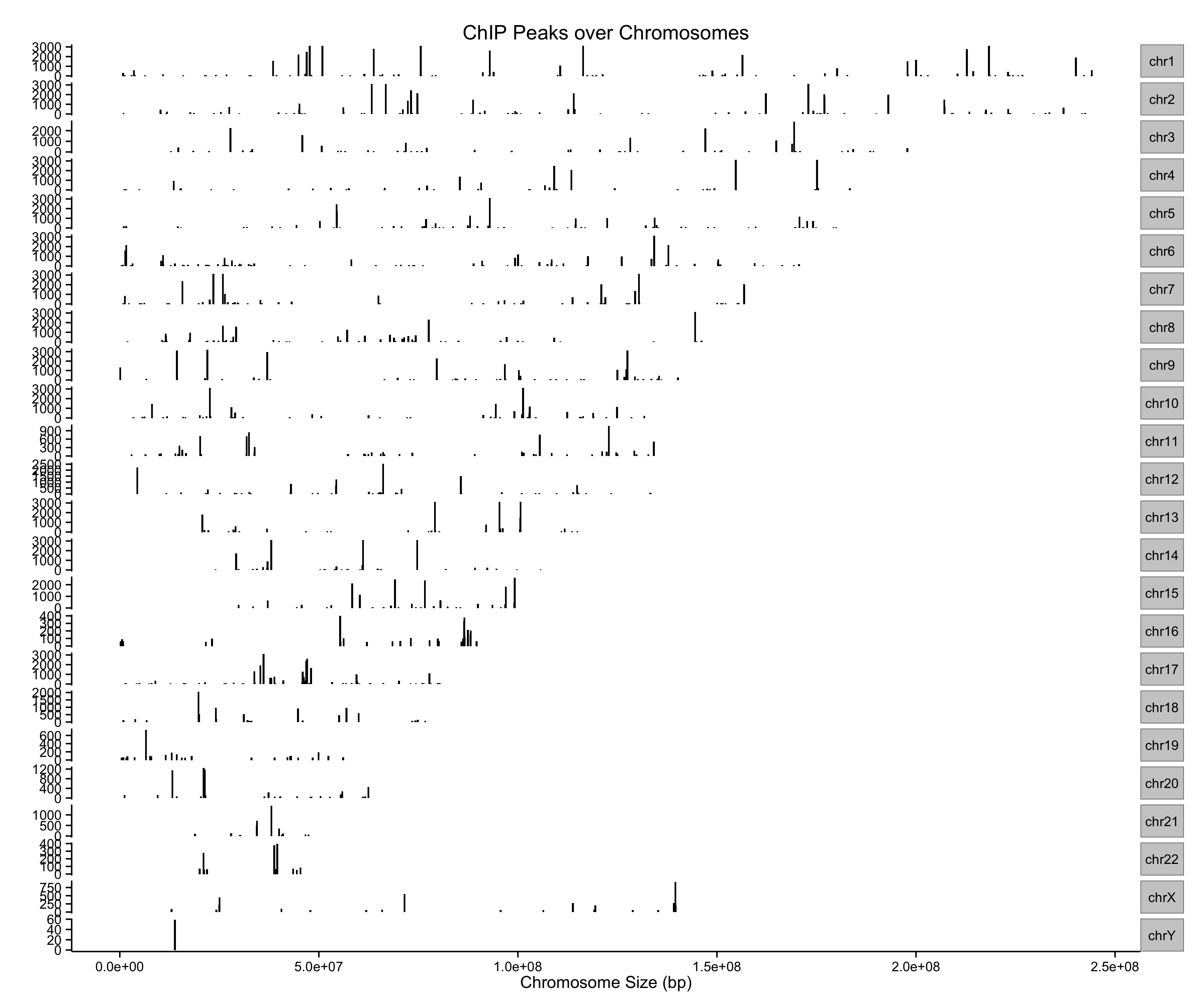
require(ChIPseeker)
files <- getSampleFiles()
peak <- readPeakFile(files[[4]])
peak[1:2,]
## GRanges with 2 ranges and 2 metadata columns:
##       seqnames           ranges strand |          V4        V5
##          <Rle>        <IRanges>  <Rle> |    <factor> <numeric>
##   [1]     chr1 [815825, 818154]      * | MACS_peak_1     113.1
##   [2]     chr1 [894175, 895222]      * | MACS_peak_2      51.0
##   ---
##   seqlengths:
##     chr1 chr10 chr11 chr12 chr13 chr14 ...  chr7  chr8  chr9  chrX  chrY
##       NA    NA    NA    NA    NA    NA ...    NA    NA    NA    NA    NA
Power
plotChrCov(peak, weightCol="V5")
Power
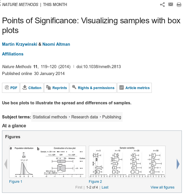
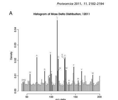
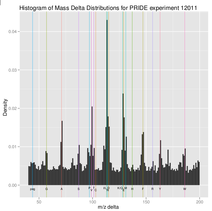
Flexibility
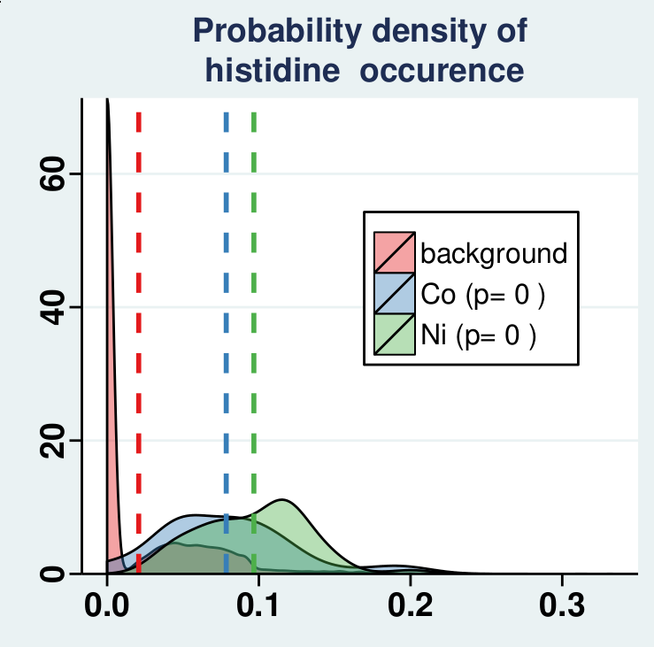
Flexibility
Proteomics. 2011, 11(11):2182-94.
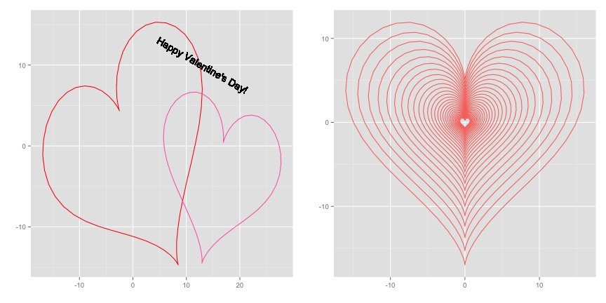
Fun
Fun
woo your girl/boy friend
Outlines
Data and Mapping
Geometric
Scale
Layer
Facet
Theme
Data and Mapping
- ggplot - The main function where you specify the dataset and variables to plot
- aes - aesthetics
- shape, transparency (alpha), color, fill, linetype.
Geometric
- geoms - geometric objects
- geom_point(), geom_bar(), geom_density(), geom_line(), geom_area()
The iris dataset
data(iris)
head(iris)
##   Sepal.Length Sepal.Width Petal.Length Petal.Width Species
## 1          5.1         3.5          1.4         0.2  setosa
## 2          4.9         3.0          1.4         0.2  setosa
## 3          4.7         3.2          1.3         0.2  setosa
## 4          4.6         3.1          1.5         0.2  setosa
## 5          5.0         3.6          1.4         0.2  setosa
## 6          5.4         3.9          1.7         0.4  setosa
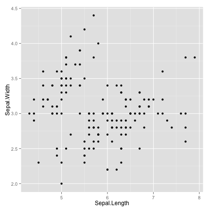
scatter plot
ggplot(data = iris, aes(x = Sepal.Length, y = Sepal.Width)) + geom_point()
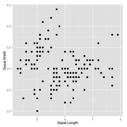
increase the size
ggplot(data = iris, aes(x = Sepal.Length, y = Sepal.Width)) + geom_point(size=3)
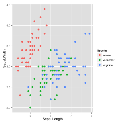
add color
ggplot(data = iris, aes(x = Sepal.Length, y = Sepal.Width, color=Species)) +
         geom_point(size=3)
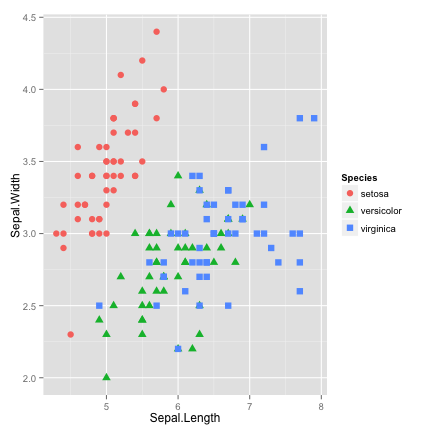
differentiate points by shape
ggplot(data = iris, aes(x = Sepal.Length, y = Sepal.Width, color=Species)) +
        geom_point(aes(shape=Species), size=3)
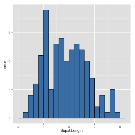
histogram
ggplot(data=iris) +
geom_histogram(aes(x=Sepal.Length), binwidth=0.2, fill="steelblue", color="black")
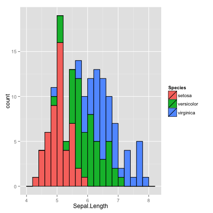
fill by Species
ggplot(data=iris) +
geom_histogram(aes(x=Sepal.Length, fill=Species), binwidth=0.2, color="black")
the diamonds dataset
data(diamonds)
set.seed(42)
dsmall <- diamonds[sample(nrow(diamonds), 1000), ]
head(dsmall)
##       carat       cut color clarity depth table price    x    y    z
## 49345  0.71 Very Good     H     SI1  62.5    60  2096 5.68 5.75 3.57
## 50545  0.79   Premium     H     SI1  61.8    59  2275 5.97 5.91 3.67
## 15434  1.03     Ideal     F     SI1  62.4    57  6178 6.48 6.44 4.03
## 44792  0.50     Ideal     E     VS2  62.2    54  1624 5.08 5.11 3.17
## 34614  0.27     Ideal     E     VS1  61.6    56   470 4.14 4.17 2.56
## 27998  0.30   Premium     E     VS2  61.7    58   658 4.32 4.34 2.67
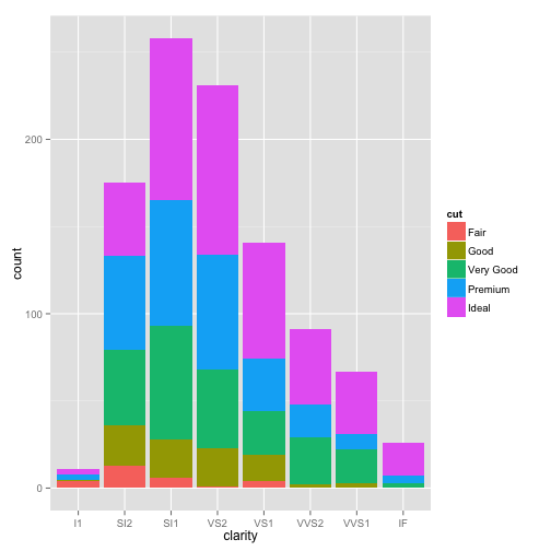
barplot
ggplot(dsmall, aes(x=clarity, fill=cut)) + geom_bar()
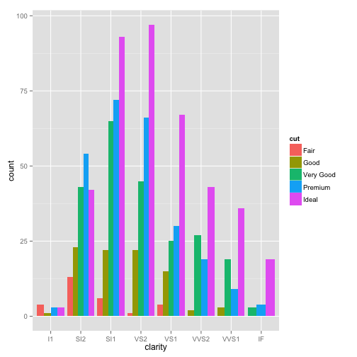
side-by-side barplot
ggplot(dsmall, aes(x=clarity, fill=cut)) + geom_bar(position="dodge")
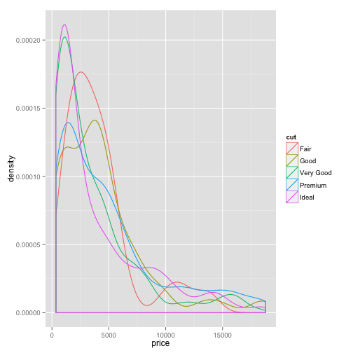
density plot
ggplot(dsmall)+geom_density(aes(x=price, colour=cut))
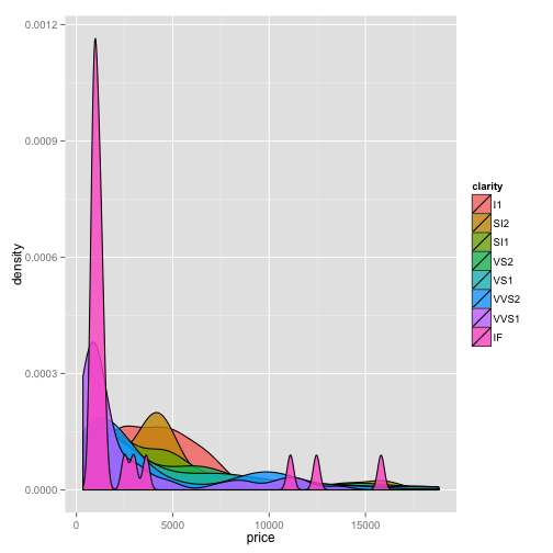
density plot
ggplot(dsmall)+geom_density(aes(x=price, fill=clarity), alpha=0.8)
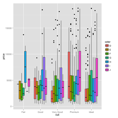
boxplot
ggplot(dsmall)+geom_boxplot(aes(x=cut, y=price,fill=color))
the climate dataset
climate <- read.csv("data/climate.csv")
head(climate)
##     X   Source Year Anomaly1y Anomaly5y Anomaly10y Unc10y
## 1 102 Berkeley 1901        NA        NA     -0.162  0.109
## 2 103 Berkeley 1902        NA        NA     -0.177  0.108
## 3 104 Berkeley 1903        NA        NA     -0.199  0.104
## 4 105 Berkeley 1904        NA        NA     -0.223  0.105
## 5 106 Berkeley 1905        NA        NA     -0.241  0.107
## 6 107 Berkeley 1906        NA        NA     -0.294  0.106
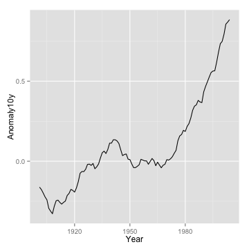
line plot
p <- ggplot(climate, aes(Year, Anomaly10y)) + geom_line()
p
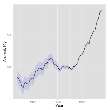
line plot with confidence interval
p + geom_ribbon(aes(ymin = Anomaly10y - Unc10y,
        ymax = Anomaly10y + Unc10y), fill = "blue", alpha = .1)
Scale
- Define how your data will be plotted
- continuous, discrete, log
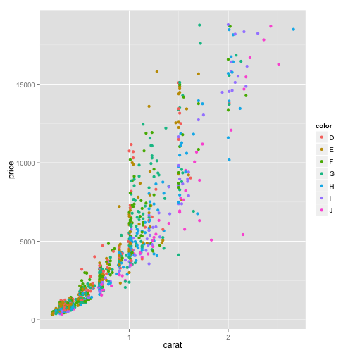
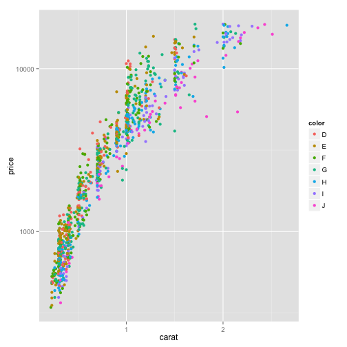
scatter plot of price vs carat
ggplot(dsmall, aes(x=carat, y=price, color=color))+geom_point()
transform y axis in log scale
ggplot(dsmall, aes(x=carat, y=price, color=color))+geom_point() + scale_y_log10()
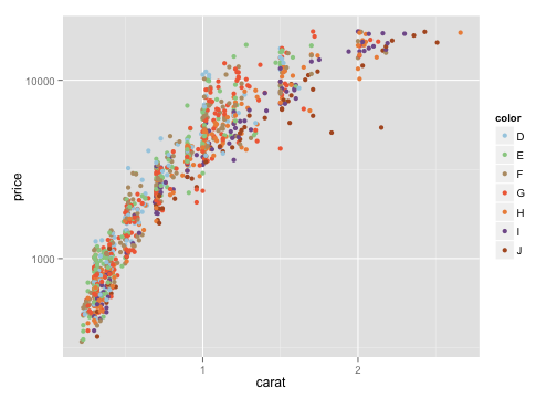
manual color scale
cols= c("#A6CEE3", "#99CD91", "#B89B74", "#F06C45", "#ED8F47", "#825D99", "#B15928")
ggplot(dsmall, aes(x=carat, y=price, color=color))+geom_point() +
      scale_y_log10() + scale_color_manual(values=cols)
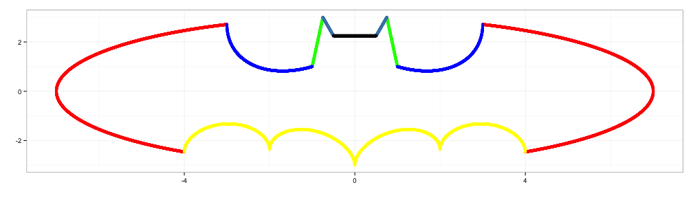
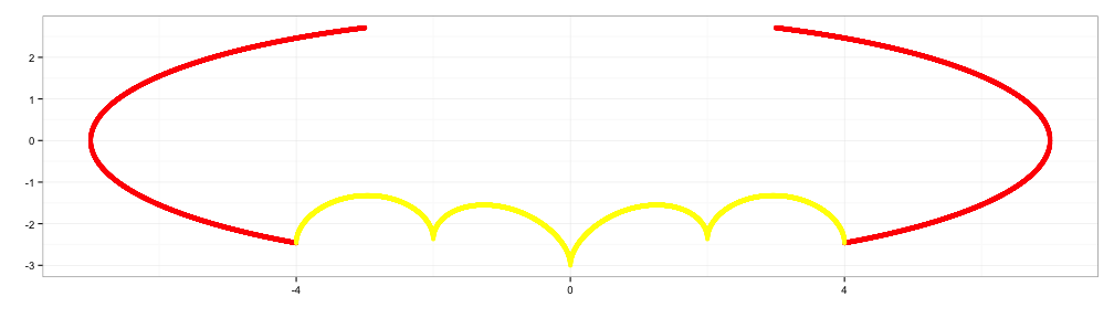
Layer
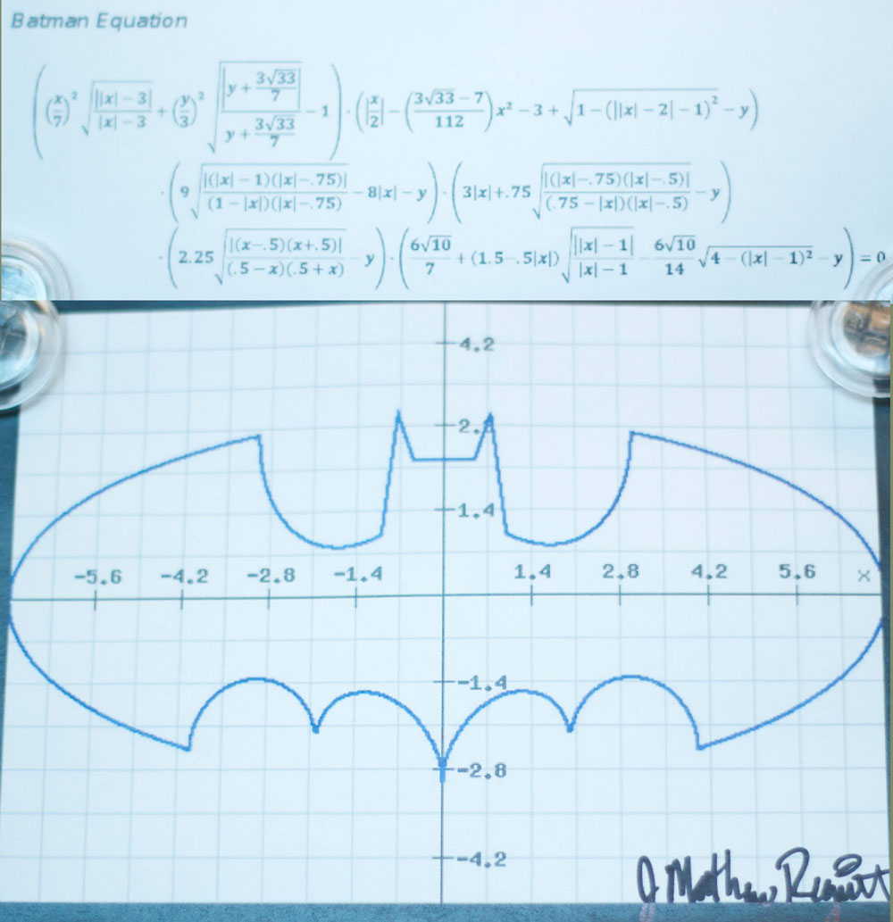
f1 <- function(x) {
y1 <- 3*sqrt(1-(x/7)^2)
y2 <- -3*sqrt(1-(x/7)^2)
y <- c(y1,y2)
d <- data.frame(x=x,y=y)
d <- d[d$y > -3*sqrt(33)/7,]
return(d)
}
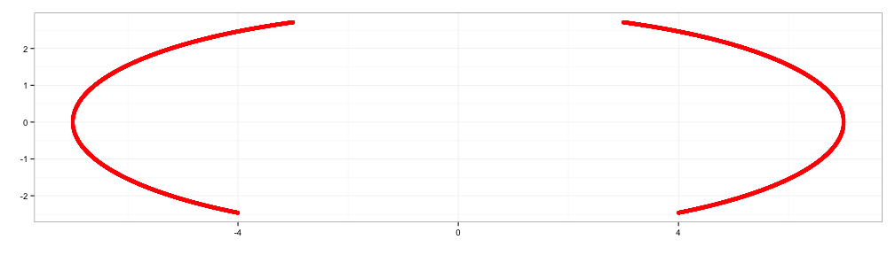
x1 <- c(seq(3, 7, 0.001), seq(-7, -3, 0.001))
d1 <- f1(x1)
p1 <- ggplot(d1,aes(x,y)) + geom_point(color="red") +xlab("") + ylab("") + theme_bw()
p1
x2 <- seq(-4,4, 0.001)
y2 <- abs(x2/2)-(3*sqrt(33)-7)*x2^2/112-3 + sqrt(1-(abs(abs(x2)-2)-1)^2)
d2 <- data.frame(x2=x2, y2=y2)
p2 <- p1 + geom_point(data=d2, aes(x=x2,y=y2), color="yellow")
p2
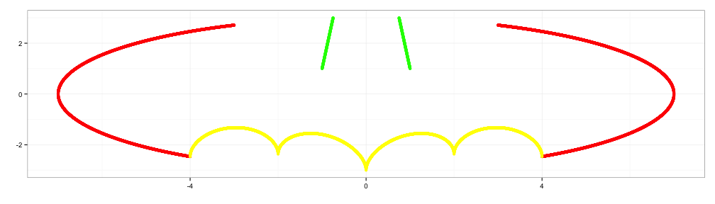
x3 <- c(seq(0.75,1,0.001), seq(-1,-0.75,0.001))
y3 <- 9-8*abs(x3)
d3 <- data.frame(x3=x3, y3=y3)
p3 <- p2+geom_point(data=d3, aes(x=x3,y=y3), color="green")
p3
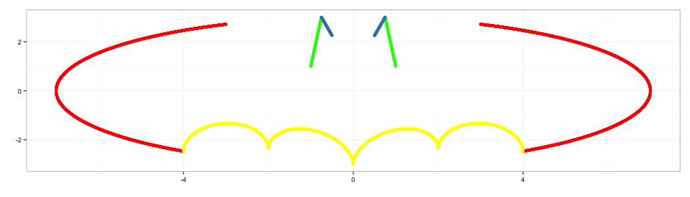
x4 <- c(seq(0.5,0.75,0.001), seq(-0.75,-0.5,0.001))
y4 <- 3*abs(x4)+0.75
d4 <- data.frame(x4=x4,y4=y4)
p4 <- p3+geom_point(data=d4, aes(x=x4,y=y4), color="steelblue")
p4
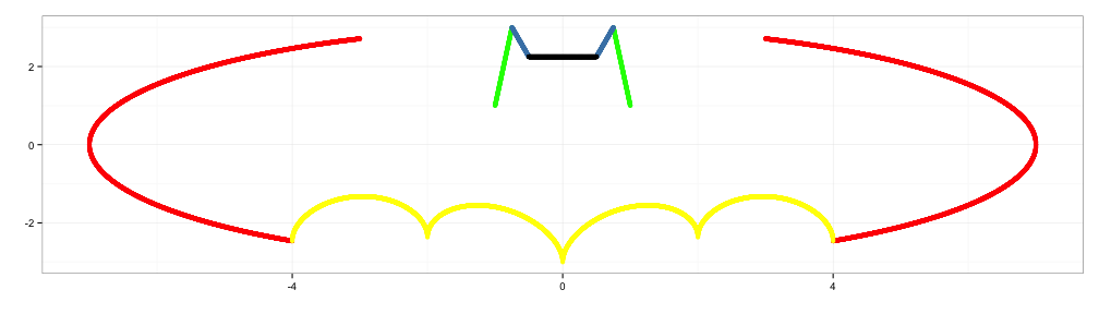
x5 <- seq(-0.5,0.5,0.001)
y5 <- rep(2.25,length(x5))
d5 <- data.frame(x5=x5,y5=y5)
p5 <- p4+geom_point(data=d5, aes(x=x5,y=y5))
p5
x6 <- c(seq(-3,-1,0.001), seq(1,3,0.001))
y6 <- 6 * sqrt(10)/7 +
    (1.5 - 0.5 * abs(x6)) * sqrt(abs(abs(x6)-1)/(abs(x6)-1)) -
    6 * sqrt(10) * sqrt(4-(abs(x6)-1)^2)/14
d6 <- data.frame(x6=x6,y6=y6)
d6 <- d6[-which(is.na(d6[,2])), ]
p6 <- p5+geom_point(data=d6,aes(x=x6,y=y6), colour="blue")
p6

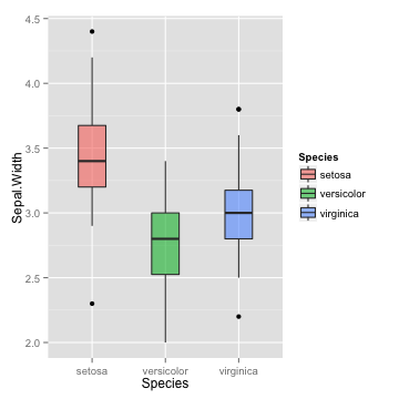
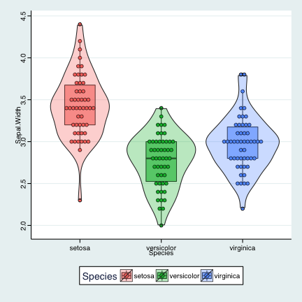
boxplot
p <- ggplot(iris, aes(x=Species, y=Sepal.Width, fill=Species)) +
     geom_boxplot(alpha=0.6, width=0.5)
p
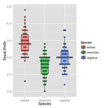
boxplot with data points
p <- p + geom_dotplot(binaxis="y", stackdir="center", position="dodge", dotsize=0.5)
p
## stat_bindot: binwidth defaulted to range/30. Use 'binwidth = x' to adjust this.
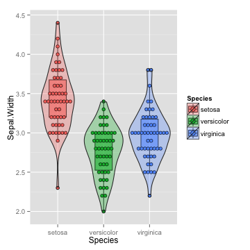
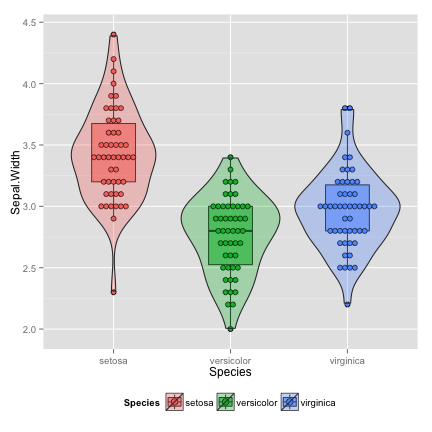
violin: add density curve
vp <- p+geom_violin(alpha=0.3)
vp
## stat_bindot: binwidth defaulted to range/30. Use 'binwidth = x' to adjust this.
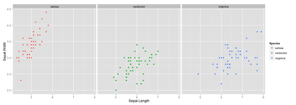
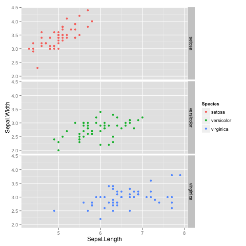
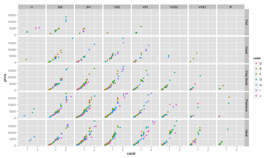
Facet
ggplot(iris, aes(Sepal.Length, Sepal.Width, color = Species)) +
         geom_point() + facet_grid(.~Species)
ggplot(iris, aes(Sepal.Length, Sepal.Width, color = Species)) +
         geom_point() + facet_grid(Species~.)
ggplot(dsmall, aes(carat, price, color=color)) +
        geom_point() +facet_grid(cut~clarity)
Theme
- A great way to define custom plots
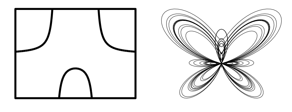
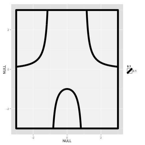
The JIONG (囧)
f <- function(x) 1/(x^2-1)
x <- seq(-3,3, by=0.001)
y <- f(x)
d <- data.frame(x=x,y=y)

p <- ggplot()
p <- p+geom_rect(fill = "white",color="black",size=3,
     aes(NULL, NULL,xmin=-3, xmax=3,
     ymin=-3,ymax=3, alpha=0.1))

p <- p + geom_line(data=d, aes(x,y), size=3)+ylim(-3,3)
p
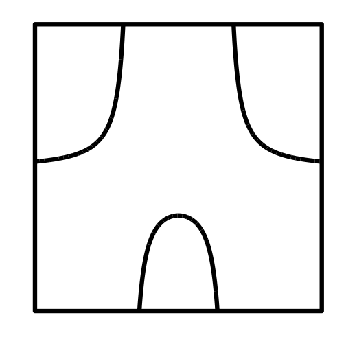
all decoration are modifiable
theme_null <- function() {
    theme_bw() %+replace%
    theme(axis.text.x=element_blank(),
    axis.text.y=element_blank(),
    legend.position="none",
    panel.grid.minor=element_blank(),
    panel.grid.major=element_blank(),
    panel.background=element_blank(),
    axis.ticks=element_blank(),
    panel.border=element_blank())
}

p <- p+theme_null()+xlab("")+ylab("")
p
vp <- vp + theme(legend.position="bottom")
vp
## stat_bindot: binwidth defaulted to range/30. Use 'binwidth = x' to adjust this.
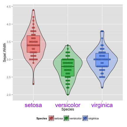
vp <- vp + theme(axis.text.x = element_text(colour = "purple",
        size = 20))
vp
## stat_bindot: binwidth defaulted to range/30. Use 'binwidth = x' to adjust this.
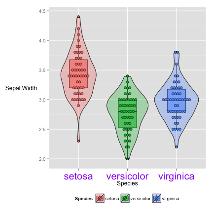
vp + theme(axis.title.y = element_text(angle = 0))
## stat_bindot: binwidth defaulted to range/30. Use 'binwidth = x' to adjust this.
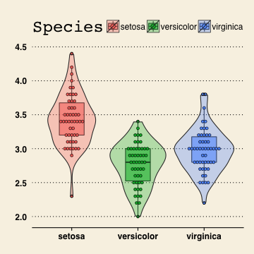
many pre-defined theme
wall street journal
require(ggthemes)
vp+theme_wsj()
## stat_bindot: binwidth defaulted to range/30. Use 'binwidth = x' to adjust this.
Stata theme
vp+theme_stata()
## stat_bindot: binwidth defaulted to range/30. Use 'binwidth = x' to adjust this.
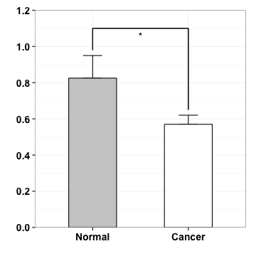
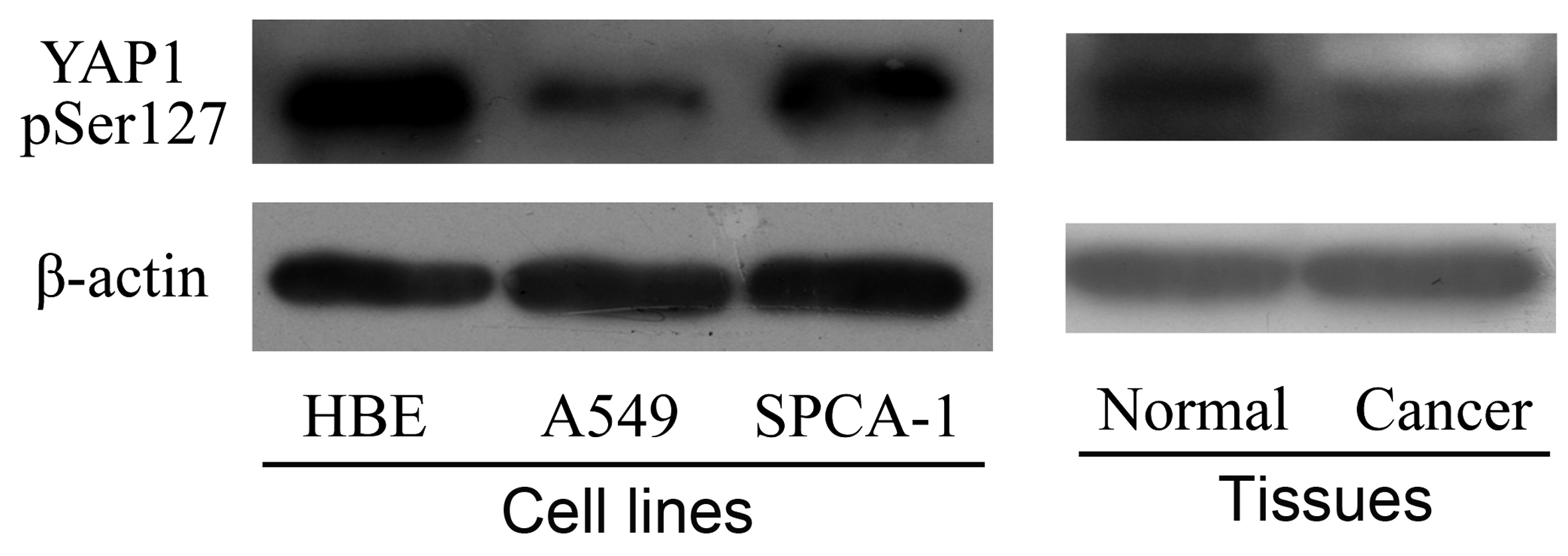
Case study
Mol Biosyst. 2011, 7(2):472-9.
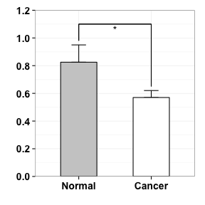
data
Normal <- c(0.83, 0.79, 0.99, 0.69)
Cancer <- c(0.56, 0.56, 0.64, 0.52)
m <- c(mean(Normal), mean(Cancer))
s <- c(sd(Normal), sd(Cancer))
d <- data.frame(V=c("Normal", "Cancer"), mean=m, sd=s)
d$V <- factor(d$V, levels=c("Normal", "Cancer"))
d
##        V  mean      sd
## 1 Normal 0.825 0.12477
## 2 Cancer 0.570 0.05033
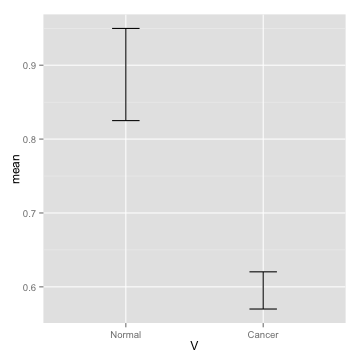
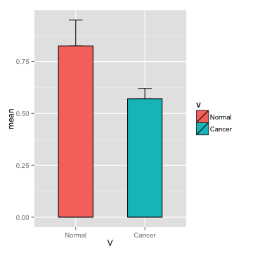
mapping & geometric
p <- ggplot(d, aes(V, mean, fill=V, width=.5))
p <- p+geom_errorbar(aes(ymin=mean, ymax=mean+sd, width=.2),
                     position=position_dodge(width=.8))
p
geometric & layer
p <- p + geom_bar(stat="identity", position=position_dodge(width=.8), colour="black")
p
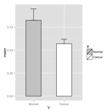
scale
p <- p + scale_fill_manual(values=c("grey80", "white"))
p
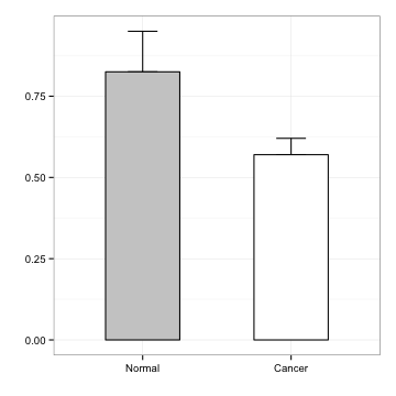
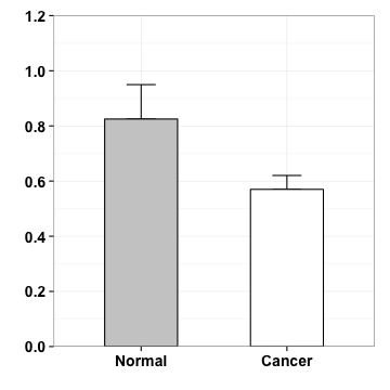
theme
p <- p + theme_bw() +theme(legend.position="none") + xlab("") + ylab("")
p
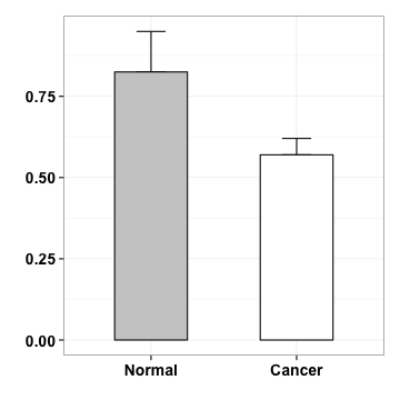
theme
p <- p + theme(axis.text.x = element_text(face="bold", size=14),
               axis.text.y = element_text(face="bold", size=14))
p
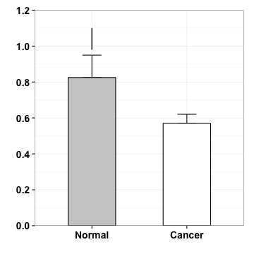
scale
p <- p+scale_y_continuous(expand=c(0,0), limits=c(0, 1.2), breaks=seq(0, 1.2, by=.2))
p
geometric
p <- p+geom_segment(aes(x=1, y=.98, xend=1, yend=1.1))
p
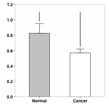
geometric
p <- p+geom_segment(aes(x=2, y=.65, xend=2, yend=1.1))
p
geometric
p <- p+geom_segment(aes(x=1, y=1.1, xend=2, yend=1.1))
p
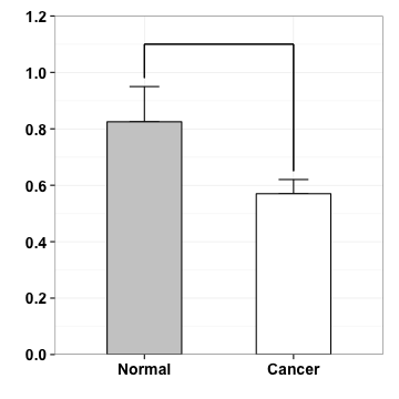
annotation
p <- p + annotate("text", x=1.5, y=1.06, label="*")
p