
covplot supports GRangesList
To answer the issue, I extend the covplot function to support viewing coverage of a list of GRanges objects or bed files.
library(ChIPseeker)
files <- getSampleFiles()
peak=GenomicRanges::GRangesList(CBX6=readPeakFile(files[[4]]),
                                CBX7=readPeakFile(files[[5]]))

p <- covplot(peak)
print(p)
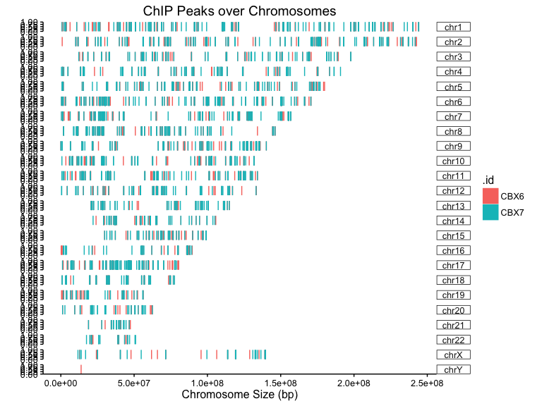
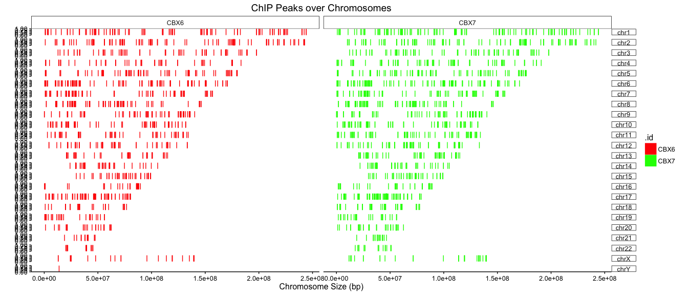
By default, The coverage plots are merged together with different colors. Users can separate them to different panels using facet_grid.
library(ggplot2)
col <- c(CBX6='red', CBX7='green')
p + facet_grid(chr ~ .id) + scale_color_manual(values=col) + scale_fill_manual(values=col)
Citation
Yu G, Wang LG and He QY*. ChIPseeker: an R/Bioconductor package for ChIP peak annotation, comparison and visualization. Bioinformatics 2015, 31(14):2382-2383.
