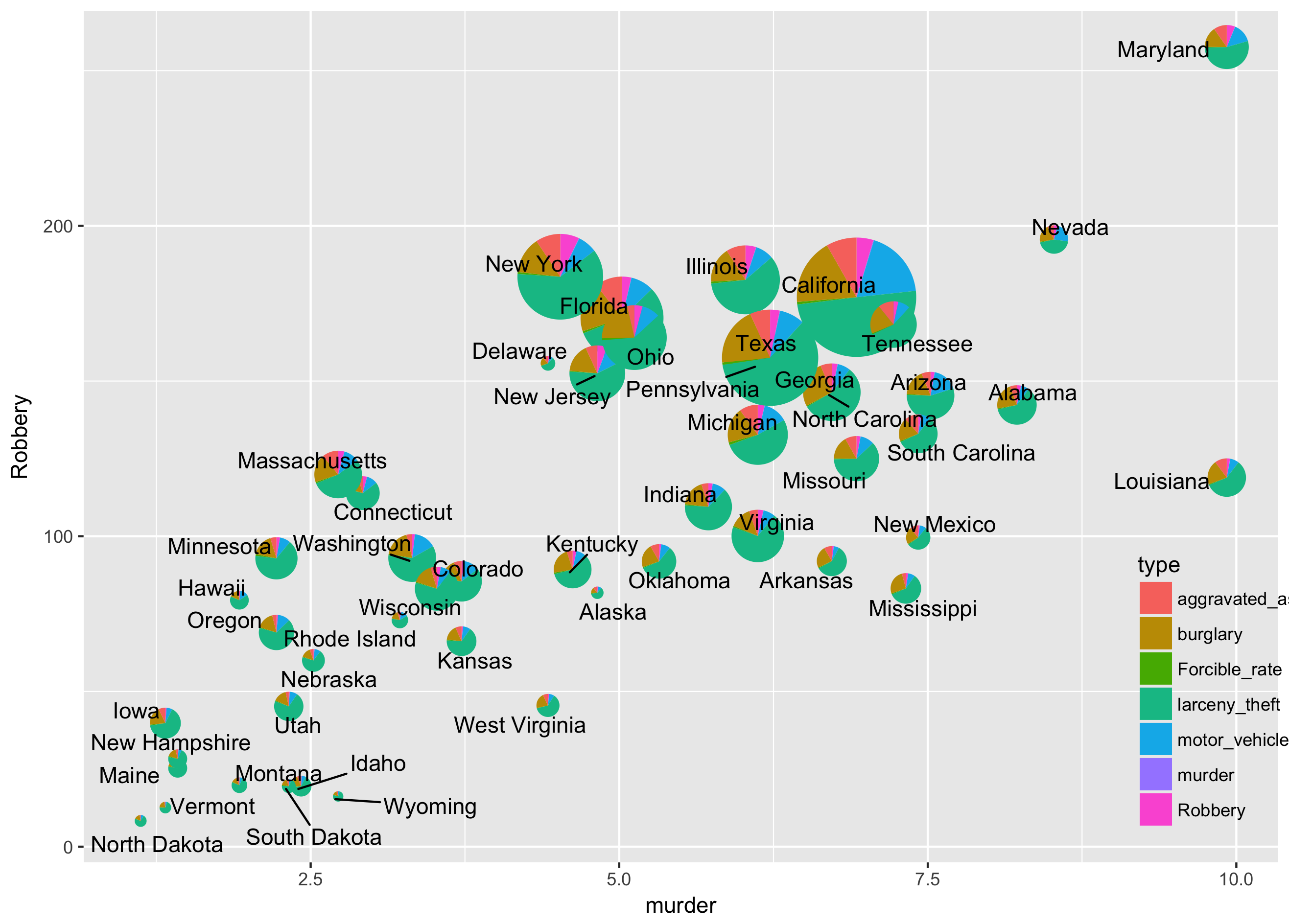
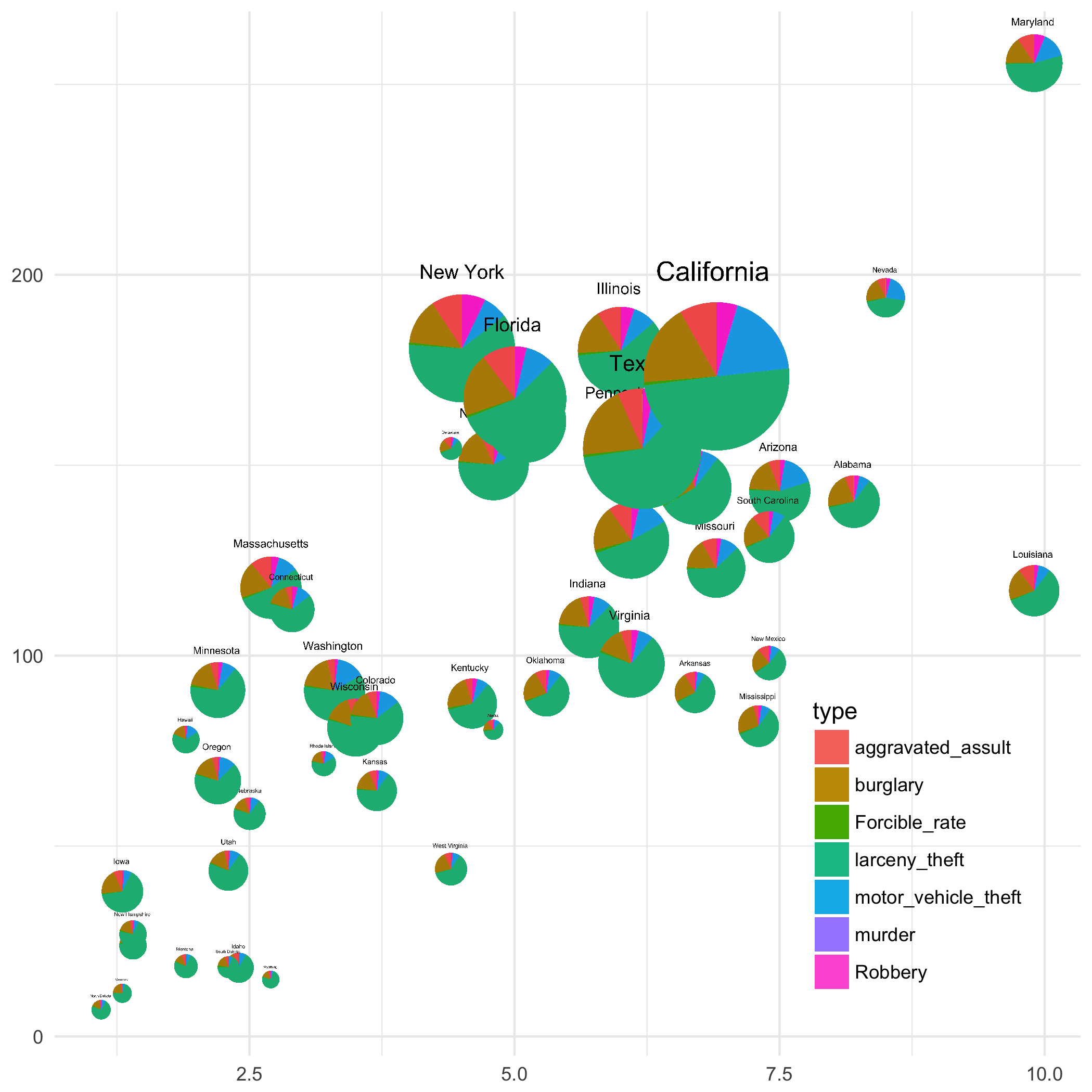
饼图版气泡图
在《ggimage:ggplot2中愉快地使用图片》一文中,我展示了「嵌套式绘图」,中间生成了多个饼图,再用这些产生的饼图用于做图,绘制出饼图版的气泡图:
当时还通过每次只画一个州的数据,来演示制作动图:
大家应该对下面Hans Rosling的动态气泡图不陌生,这其实是我在对Hans Rosling致敬。

ggimage包对这种图中套图的做法,不需要中间产生图片也是可以完成的。因为我们有geom_subview图层,直接可以操作ggplot对象。
首先我们载入所需的包,并读入数据:
library(gtable)
library(ggplot2)
library(tidyr)
library(tibble)
library(ggimage)
library(ggrepel)

crime <- read.table("http://datasets.flowingdata.com/crimeRatesByState2005.tsv",
                  header=TRUE, sep="\t", stringsAsFactors=F)
定义一个plot_pie函数,用于画饼图,并返回ggplot对象。将这一函数应用于crime数据每一行,并把图对象又存回crime中。
plot_pie <- function(i) {
    df <- gather(crime[i,], type, value, murder:motor_vehicle_theft)
    ggplot(df, aes(x=1, value,fill=type)) +
        geom_col() + coord_polar(theta = 'y') +
        ggtitle(crime[i, "state"]) +
        theme_void() + theme_transparent() +
        theme(legend.position = "none",
              plot.title = element_text(size=rel(6), hjust=0.5))
}

crime <- as_data_frame(crime)

crime$pie <- lapply(1:nrow(crime), plot_pie)
我们根据人口,按照比例来计算饼图的大小,并且抽离出饼图的图例:
radius <- sqrt(crime$population / pi)
radius <- radius/max(radius)

crime$width <- diff(range(crime$murder)) * 0.2 * radius
crime$height <- diff(range(crime$Robbery)) * 0.2 * radius

leg1 <- gtable_filter(
    ggplot_gtable(
        ggplot_build(plot_pie(1) + theme(legend.position="right"))
    ), "guide-box")
最后是出图,用geom_subview加图例,再用geom_subview加饼图,最后加geom_text_repel图层,写上州名。
p <- ggplot(crime, aes(murder, Robbery)) + geom_subview(leg1, x=10, y=50) +
    geom_subview(crime$pie, crime$murder, crime$Robbery, width=crime$width, height=crime$height) +
    geom_text_repel(aes(label=state))

ggsave(p, file="bubble_pie.png")