
你还在愁毕业?隔壁实验室的小哥从网上抄了几十行代码打了个R包,发了SCI,毕业了!
你是否对《R包辣鸡之CorMut》之篇还有印象?没有的话,快点打开阅读一下,这文章让作者毕业了,毕竟发表的是一篇Bioinformatics。
《[连载3]:辣眼睛,一篇抄袭引发的系列血案!》,而这一篇文章中揭露了某讲师抄袭了两个R包,晋升副教授了!文章中还稍带了另外一个学生也是抄袭,当然也发表了SCI,也毕业了。
今天讲另外一个R包,它做下面的事情:
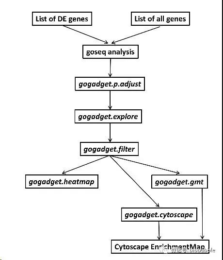
当然前面的事情是goseq干的,它的功能就是衔接了goseq的输出,让我们还看看它每一步都在做什么。
gogadget.p.adjust
gogadget.p.adjust <- function(x, method = "BH") {
    adjustedP <- p.adjust(x$over_represented_pvalue, method = method)
    x["adjusted_pvalue"] <- adjustedP
    return(x)
}
这一步干的事情,就是给goseq的输出加一个adjusted pvalue,仅此而已。
gogadget.explore
gogadget.explore <- function(x , nmin = 10, stepmin = 10, nmax = 100, stepmax = 100, steps = 4, cutoff = 0.05, legend = "topleft") {
    seqmin <- seq(nmin, nmin+stepmin*steps, by = stepmin)
    seqmax <- seq(nmax, nmax+stepmax*steps, by = stepmax)
    x.bar <- c()
    x.name <- c()
    for(nmin in seqmin) {
        for(nmax in seqmax) {
        x.filter <- gogadget.filter(x, cutoff = cutoff, nmin = nmin, nmax = nmax)
        cat("Filtering with min.", nmin,"and max.", nmax, "genes results in:", length(x.filter$category), "GO terms", "\n")
        x.bar <- append(x.bar, length(x.filter$category))
        x.name <- append(x.name, nmin)
        }
    }
    barplot(x.bar, ylab = "Number of GO terms", col=c(1:length(seqmax)), names = c(x.name), cex.names = 0.7,
    legend = seqmax, args.legend = list(x = legend, bty = "n", title = "Max.", cex = 0.8), xlab = "Min.")
}
这个函数就是取不同的gene set size去过滤数据,看看能留下多少结果,比如说基因集的大小在[10, 100]的情况下,过滤后有多少个结果,在[20, 100]的情况下又有多少个结果,以此类推,然后画一个柱状图,这就是所谓的结果探索了,探索是为了衔接下一步的过滤。
它的理由在于富集的结果冗余度很大,看不过来,于是过滤一下,比如说就限制在基因集[50, 100]之间吧,结果出来的数目比较少。这简直是掩耳盗铃!因为完全没有任何生物学意义的过滤。结果太多,你不是去冗余,而是随意的过滤,只为了数目少。
gogadget.filter
gogadget.filter <- function(x, cutoff = 0.05, nmin = 50, nmax = 250) {
    x.sig <- x[x[, "adjusted_pvalue"] < cutoff,]
    x.sig.filter <- x.sig[x.sig[, "numInCat"] >= nmin & x.sig[, "numInCat"] <= nmax,]
    return(x.sig.filter)
}
有了上面的解说,你该看得懂这个过滤了,一方面是p值,另一方面是指定基因集的大小进行过滤,而根据嘛,就是上面所谓的探索,就是一个柱状图,让你看什么样的基因集大小区间,出来的结果比较符合你想要的数目,真的就只是看数目,你很可能把最有用的信息都去掉,留下来一些高度冗余的,几乎没有信息量的结果。
gogadget.heatmap
gogadget.heatmap <- function(x, genes, genome, id, fetch.cats = c("GO:CC","GO:BP","GO:MF"), symm = T, trace = "none", density.info = "none", cexRow = 0.4, cexCol = 0.4, col = my_palette, margins = c(3, 11), revC = T, ...) {
    allGOs <- stack(getgo(genes, genome, id, fetch.cats = fetch.cats))
    b <- 1
    name <- list()
    name[1:length(x$category)] <- paste("var", 1:length(x$category), sep = "")
    for(a in x$category) {
        new <- allGOs[allGOs["values"] == a,]
        name[[b]] <- new$ind
        b <- b+1
    }
    m <- matrix(nrow = length(name), ncol = length(name))
    for(i in 1:length(name)) {
        for(j in 1:length(name)) {
        overlap <- name[[i]] %in% name[[j]]
        m[i,j] <- length(overlap[overlap == TRUE])
        }
    }
    GOterms <- subset(x, category == x$category, select = c(category, term))
    colnames(m) <- GOterms$category
    mp <- cor(m)
    rownames(mp) <- GOterms$term
    my_palette <- colorRampPalette(c("blue", "white", "red"))(n = 299)
    heatmap.2(mp, symm = symm, trace = trace, density.info = density.info, cexRow = cexRow, cexCol = cexCol, col = col, margins = margins, revC = revC, ...)
    mp <<- mp
}
富集到的GO,两两计算一下两个基因集overlap了多少,以此形成一个矩阵,然后对矩阵求pearson相关系数,对相关系数用heatmap.2画热图。这就是所谓对冗余GO进行层次聚类。
PS:这里犯了一个大忌,用了«-。
gogadget.cytoscape
gogadget.cytoscape <- function(x, file = "File4cytoscape.txt") {
    x.cytoscape <- x[,c("category", "term", "over_represented_pvalue", "adjusted_pvalue")]
    colnames(x.cytoscape) <- c("GO.ID", "Description", "p.Val", "FDR")
    write.table(x.cytoscape, file = file, sep = "\t", row.names = F, quote = F)
    cat(file,"is written to your working directory.\n")
}
这个就是把goseq的结果写成一个table,这样可以导入到cytoscape里去。当然光这个文件是不够的,所以需要下面这一步的文件。
gogadget.gmt
gogadget.gmt <- function(x, genes, genome, id, fetch.cats=c("GO:CC","GO:BP","GO:MF"), file = "cytoscape.gmt") {
    allGOs <- stack(getgo(genes, genome, id, fetch.cats = fetch.cats))
    newdf<-as.data.frame(cbind(x$category,x$term))
    colnames(newdf)<-c("values","term")
    reshaped <- group_by(allGOs, values) %>% summarise(genes = paste(ind, collapse = "\t"))
    reshaped.terms <- left_join(reshaped, newdf, by = "values",copy = T)
    reshaped.terms <- reshaped.terms[,c(1,3,2)]
    write.table(reshaped.terms, file = file, sep = "\t", quote = FALSE, row.names = FALSE, col.names = FALSE)
}
这个是生成gmt文件,这样有基因集的信息,和上面的输出一起,两个文件就可以通过cytoscape画enrichment map了。
然后这个包的功能就完了,而且所有代码也完了!你看到上面函数用到的getgo这些函数,是来自于goseq的,这个包并没有写工具性的函数被上面的函数所调用,它的代码真的就是这么多。
审稿吐槽
我帮他数了一下,78行代码,其实在它提交文章的时候,我就帮他数过了,66行,后来它还加了12行。
Some of gogadget’s functions were developed with help and advice from users of the Biostars (https://www.biostars.org/) and Bioconductor Support (https://support.bioconductor.org/) website.
而且作者在致谢中还感谢了网友们的帮助才有这几十行的代码。就这样一个R包,发表了SCI论文:
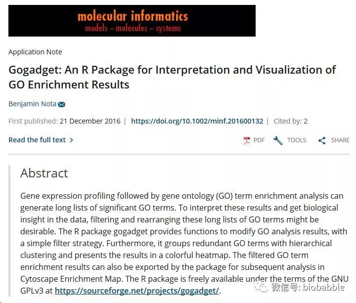
你能想象作者竟然敢把它submit到Bioinformatics上吗?而Bioinformatics的Editor竟然还送审了!想我8年前提交clusterProfiler到Bioinformatics上,起码那年头也是第一次你可以在R包里批量对多个条件做富集分析并且把结果用点图呈现出来,好比较。记住这是8年前!然后Editor直接reject,并且说你不要再提交了,我们不接受这篇文章以任何形式再次提交!我真的好受伤。
这篇gogadget的文章就是我审的稿,我直接就reject了,9月底reject,作者很快投了个小杂志,以极快的速度就被接收了:
Manuscript accepted:
02 December 2016
Manuscript received:
06 October 2016
(鉴于文章已经发表了几年,审稿的保密性和匿名性已经不重要)我当时的审稿意见是:
This R package is hosted in sourceforge. Any published package should be hosted in either Bioconductor or CRAN as they will test and build the package (ensure it’s runnable in current R release) and more easy to install.
第一点,要发表R包,最好放CRAN或Bioconductor上,起码易安装,也有人去针对当前的R版本进行测试和编译。从后面发表的文章看,作者无视我的建议。
This gogadge package is quite tiny with only 66 lines of source code and its functions are quite simple without any innovation.
改成了78行,依然是太过于简章粗暴。
For simplifying result to help interpretation, there are several tools that employ GO semantic similarity measure to remove redundant terms such as REVIGO, clusterProfiler etc. Filter by number as defined in gogadget.filter is too simply and can’t resolve the redundant issue.
指出它并不能解决问题,而且明明有更好的方案已经存在。
Heatmap and cytoscape’s enrichmap are good visualization tools for visualize related (redundant) terms but not directly solving the issue to simplify the result and help interpretation.
可视化有助于去解析结果,但并没有直接解决问题。
In my opinion, there is a better tool, RedundancyMiner, that can plot heatmap for GO terms. For enrichment map, this tool only generate txt file for cytoscape. Bioconductor package, clusterProfiler, can visualize enrichment map. It can simplify results by removing redundant terms using semantic similarity calculation followed by visualizing using enrichment map. All the functions provided by gogadget have better alternative in other software packages. This package is just too simple without innovation.
指出来所有功能都有更好的实现存在,完全没有创新。其实另一个reviewer也指出说,没有和已有的包做比较,作者选择无视,因为根本没法拉出来和别的包溜一溜啊。但凡是像我这种review的时候,打开源码一看的,它必死无疑了。
In addition, as there are many R packages that can perform GO enrichment analysis, such as GOstats, clusterProfiler, gage, geneAnswer, etc, we expect a package that designed for helping interpreting and visualizing result to work with other R packages to help users integrate their tools with existing pipeline. But unfortunately, gogadge only work with goseq.
最后指出一点,作为一个目标是帮助解析结果的包,最好能够支持不同的软件输出,这样可以被整合到各种已有的pipeline中,而不是只针对一个goseq,显然作者也无视这一建议。
在被拒稿之后,作者根本就无视审稿意见,不做提升,立马换一个杂志投,然后小杂志一下就中了,影响因子1.96,华丽丽地可以毕业了。靠着网友的解答,整理一下小代码,打个包,包装一下,就这样发表了。
代码靠网友
Some of gogadget’s functions were developed with help and advice from users of the Biostars (https://www.biostars.org/) and Bioconductor Support (https://support.bioconductor.org/) website.
在这里以gogadget.gmt为例,这个函数从goseq中提取基因的GO注释(用的是goseq中的函数getgo),目标是要写出一个gmt格式的文件,一个GO是一column,另一个column是对应的所有基因ID,以tab分隔,好了,这么简单的事情,作者不知道怎么搞,于是在Bioconductor上问网友(https://support.bioconductor.org/p/77134/)。
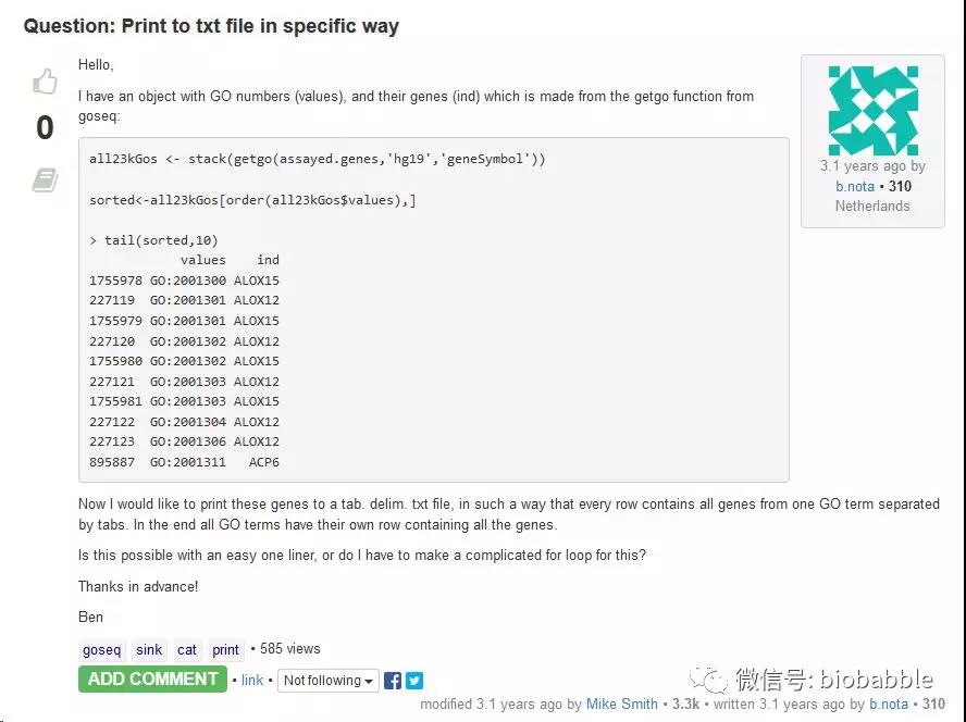
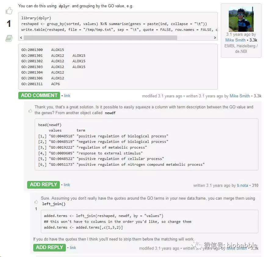
网友给出代码,天了撸,他竟然继续提问,如果要用GO Description而不是Term,该怎么搞,这就是简单的merge而已啊,网友给出的是dplyr的代码,告诉他用left_join。
让我们再翻出来gogadget.gmt函数:
gogadget.gmt <- function(x, genes, genome, id, fetch.cats=c("GO:CC","GO:BP","GO:MF"), file = "cytoscape.gmt") {
    allGOs <- stack(getgo(genes, genome, id, fetch.cats = fetch.cats))
    newdf<-as.data.frame(cbind(x$category,x$term))
    colnames(newdf)<-c("values","term")
    reshaped <- group_by(allGOs, values) %>% summarise(genes = paste(ind, collapse = "\t"))
    reshaped.terms <- left_join(reshaped, newdf, by = "values",copy = T)
    reshaped.terms <- reshaped.terms[,c(1,3,2)]
    write.table(reshaped.terms, file = file, sep = "\t", quote = FALSE, row.names = FALSE, col.names = FALSE)
}
后面几行和网友回答中给出的(下面的)代码,是不是一模一样?
reshaped <- group_by(sorted, values) %>% summarise(genes = paste(ind, collapse = "\t"))
added.terms <- left_join(reshaped, newdf, by = "values")
## this won't have to columns in the order you'd like, so change them
added.terms <- added.terms[,c(1,3,2)]
write.table(added.terms, file = "/tmp/tmp.txt", sep = "\t", quote = FALSE, row.names = FALSE, col.names = FALSE)
这只是我搜了一下Bioconductor support site之后的发现,如果你有心去搜biostar的话,你会发现更多的代码来自于网友。
吐槽归吐槽,写这篇文章是为了跟大家讲,小文章真的挺容易发表的,但凡用点心的研究生,都不应该存在毕业的问题。隔壁实验室都人手一篇了,你还在愁啊愁!赶紧学习如何写R包。只有写不出R包,没有写出来发表不了的!简单如本文,代码还来自于网友,发表了,硬伤如《R包辣鸡之CorMut》的,也发表了,甚至于开头讲到的某讲师靠晋升副教授的,也是靠发表了几篇抄袭的R包(科研无捷径,像这种无耻到连裤衩都不要的故事,请大家一起来鄙视)。
你即将要写的R包,也会发表的!
