Chapter 4 Visualization and annotation of phylogenetic trees: ggtree
4.1 Introduction
There are many software packages and webtools that are designed for displaying phylogenetic trees, such as TreeView (Page 2002), FigTree7, TreeDyn (Chevenet et al. 2006), Dendroscope (Huson and Scornavacca 2012), EvolView (Z. He et al. 2016) and iTOL (Letunic and Bork 2007), etc.. Only several of them, such as FigTree, TreeDyn and iTOL, allow users to annotate the trees with coloring branches, highlighted clades and tree features. However, their pre-defined annotating functions are usually limited to some specific phylogenetic data. As phylogenetic trees become more widely used in multidisciplinary studies, there is an increasing need to incorporate various types of the phylogenetic covariates and other associated data from different sources into the trees for visualizations and further analyses. For instance, influenza virus has a wide host range, diverse and dynamic genotypes and characteristic transmission behaviors that are mostly associated with the virus evolution and essentially among themselves. Therefore, in addition to standalone applications that focus on each of the specific analysis and data type, researchers studying molecular evolution need a robust and programmable platform that allows the high levels integration and visualization of many of these different aspects of data (raw or from other primary analyses) over the phylogenetic trees to identify their associations and patterns.
To fill this gap, we developed ggtree, a package for the R programming language (R Core Team 2016) released under the Bioconductor project (Gentleman et al. 2004). The ggtree is built to work with phylogenetic data object generated by treeio, and display tree graphics with ggplot2 package (Wickham 2016) that was based on the grammar of graphics (Wilkinson et al. 2005).
The R language is increasingly being used in phylogenetics. However, a comprehensive package, designed for viewing and annotating phylogenetic trees, particularly with complex data integration, is not yet available. Most of the R packages in phylogenetics focus on specific statistical analyses rather than viewing and annotating the trees with more generalized phylogeny-associated data. Some packages, including ape (Paradis, Claude, and Strimmer 2004) and phytools (Revell 2012), which are capable of displaying and annotating trees, are developed using the base graphics system of R. In particular, ape is one of the fundamental package for phylogenetic analysis and data processing. However, the base graphics system is relatively difficult to extend and limits the complexity of tree figure to be displayed. OutbreakTools (Jombart et al. 2014) and phyloseq (McMurdie and Holmes 2013) extended ggplot2 to plot phylogenetic trees. The ggplot2 system of graphics allows rapid customization and exploration of design solutions. However these packages were designed for epidemiology and microbiome data respectively and did not aim to provide a general solution for tree visualization and annotation. The ggtree package also inherits versatile properties of ggplot2, and more importantly allows constructing complex tree figures by freely combining multiple layers of annotations using the tree associated data imported from different sources (importation using treeio package is detailed in Chapter 2).
4.2 Methods and Materials
The ggtree package is designed for annotating phylogenetic trees with their associated data of different types and from various sources. These data could come from users or analysis programs, and might include evolutionary rates, ancestral sequences, etc. that are associated with the taxa from real samples, or with the internal nodes representing hypothetic ancestor strain/species, or with the tree branches indicating evolutionary time courses. For instance, the data could be the geographic positions of the sampled avian influenza viruses (informed by the survey locations) and the ancestral nodes (by phylogeographic inference) in the viral gene tree (Lam et al. 2012).
The ggtree supports ggplot2’s graphical language, which allows high level of customization, is intuitive and flexible. It is notable that ggplot2 itself does not provide low-level geometric objects or other support for tree-like structures, and hence ggtree is a useful extension on that regard. Even though the other two phylogenetics-related R packages, OutbreakTools and phyloseq, are developed based on ggplot2, the most valuable part of ggplot2 syntax - adding layers of annotations - is not supported in these packages. For example, if we have plotted a tree without taxa labels, OutbreakTools and phyloseq provide no easy way for general R users, who have little knowledge about the infrastructures of these packages, to add a layer of taxa labels. The ggtree extends ggplot2 to support tree objects by implementing a geometric layer, geom_tree, to support visualizing tree structure. In ggtree, viewing a phylogenetic tree is relatively easy, via the command ggplot(tree_object) + geom_tree() + theme_tree() or ggtree(tree_object) for short. Layers of annotations can be added one by one via the + operator. To facilitate tree visualization, ggtree provides several geometric layers, including geom_treescale for adding legend of tree branch scale (genetic distance, divergence time, etc.), geom_range for displaying uncertainty of branch lengths (confidence interval or range, etc.), geom_tiplab for adding taxa label, geom_tipoint and geom_nodepoint for adding symbols of tips and internal nodes, geom_hilight for highlighting a clade with rectangle, and geom_cladelabel for annotating a selected clade with a bar and text label, etc.. A full list of geometric layers provided by ggtree are summarized in Table 4.1.
4.3 Results
4.3.1 Features
The ggtree supports displaying phylogram and cladogram (Figure 4.1) and can visualize a tree with different layouts, including rectangular, slanted, circular, fan, unrooted, time-scale and two-dimensional tree.
The ggtree allows tree covariates stored in tree object to be used directly in tree visualization and annotation. These covariates can be meta data of the sampling species/sequences used in the tree, statistical analysis or evolutionary inferences of the tree (e.g. divergence time inferred by BEAST or ancestral sequences inferred by HyPhy, etc.). These numerical or categorical data can be used to color branches or nodes of the tree, displayed on the tree with original values or mapping to different symbols. In ggtree, users can add layers to highlight the selected clades, and to label clades or annotate the tree with symbols of different shapes and colors, etc. (more details in Section 3.3.3).
Comparing to other phylogenetic tree visualizing packages, ggtree excels at exploring the tree structure and related data visually. For example, a complex tree figure with several annotation layers can be transferred to a new tree object without step-by-step re-creation. An operator, %<%, was created for such operation - to update a tree figure with a new tree object. Branch length can be re-scaled using other numerical variable (as shown in Figure 3.4 which rescales the tree branches using dN value). Phylogenetic trees can be visually manipulated by collapsing, scaling and rotating clade. Circular and fan layout tree can be rotated by specific angle. Trees structures can be transformed from one layout to another.
The groupClade function assigns the branches and nodes under different clades into different groups. Similarly, groupOTU function assigns branches and nodes to different groups based on user-specified groups of operational taxonomic units (OTUs) that are not necessarily within a clade, but can be monophyletic (clade), polyphyletic or paraphyletic. A phylogenetic tree can be annotated by mapping different line type, size, color or shape to the branches or nodes that have been assigned to different groups.
Treeio package parses diverse annotation data from different software outputs into S4 phylogenetic data objects. The ggtree mainly utilizes these S4 objects to display and annotate the tree. There are also other R packages that defined S3/S4 classes to store phylogenetic trees with their specific associated data, including phylo4 and phylo4d defined in phylobase package, obkdata defined in OutbreakTools package, and phyloseq defined in phyloseq package. All these tree objects are also supported in ggtree and their specific annotation data can be used to annotate the tree in ggtree. Such compatibility of ggtree facilitates the integration of data and analysis results.
4.3.2 Layouts of phylogenetic tree
Viewing phylogenetic with ggtree is quite simple, just pass the tree object to ggtree function. We have developed several types of layouts for tree presentation (Figure 4.1), including rectangular (by default), slanted, circular, fan, unrooted (equal angle and daylight methods), time-scaled and 2-dimensional layouts.
Here are examples of visualizing a tree with different layouts:
library(ggtree)
set.seed(2017-02-16)
tree <- rtree(50)
ggtree(tree)
ggtree(tree, layout="slanted")
ggtree(tree, layout="circular")
ggtree(tree, layout="fan", open.angle=120)
ggtree(tree, layout="equal_angle")
ggtree(tree, layout="daylight")
ggtree(tree, branch.length='none')
ggtree(tree, branch.length='none', layout='circular')
ggtree(tree, layout="daylight", branch.length = 'none')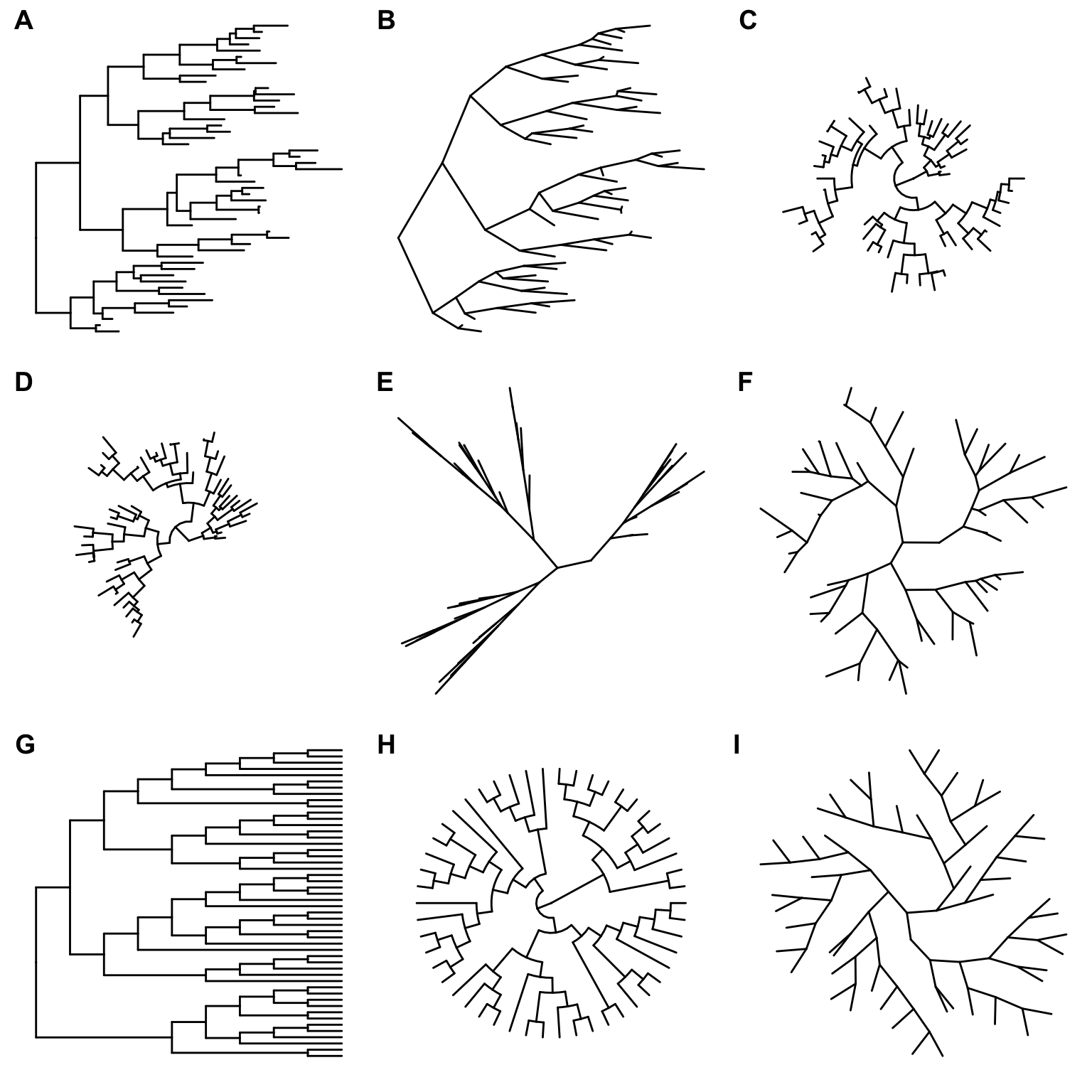
Figure 4.1: Tree layouts. Phylogram: rectangular layout (A), slanted layout (B), circular layout (C) and fan layout (D). Unrooted: equal-angle method (E) and daylight method (F). Cladogram: rectangular layout (G), circular layout (H) and unrooted layout (I). Slanted and fan layouts for cladogram are also supported.
Phylogram. Layouts of rectangular, slanted, circular and fan are supported to visualize phylogram (by default, with branch length scaled) as demonstrated in Figure 4.1A, B, C and D.
Unrooted layout. Unrooted (also called ‘radial’) layout is supported by equal-angle and daylight algorithms, user can specify unrooted layout algorithm by passing “equal_angle” or “daylight” to layout parameter to visualize the tree. Equal-angle method was proposed by Christopher Meacham in PLOTREE, which was incorporated in PHYLIP (Retief 2000). This method starts from the root of the tree and allocates arcs of angle to each subtrees proportional to the number of tips in it. It iterates from root to tips and subdivides the angle allocated to a subtree into angles for its dependent subtrees. This method is fast and was implemented in many software packages. As shown in Figure 4.1E, equal angle method has a drawback that tips are tend to be clustered together and leaving many spaces unused. The daylight method starts from an initial tree built by equal angle and iteratively improves it by successively going to each interior node and swinging subtrees so that the arcs of “daylight” are equal (Figure 4.1F). This method was firstly implemented in PAUP* (Wilgenbusch and Swofford 2003).
Cladogram. To visualize cladogram that without branch length scaling and only display the tree structure, branch.length is set to “none” and it works for all types of layouts (Figure 4.1G, H and I).
Time-scaled layout. For time-scaled tree, the most recent sampling date must be specified via the mrsd parameter and ggtree will scaled the tree by sampling (tip) and divergence (internal node) time, and a time scale axis will be displayed under the tree by default.
beast_file <- system.file("examples/MCC_FluA_H3.tree",
                          package="ggtree")
beast_tree <- read.beast(beast_file)
ggtree(beast_tree, mrsd="2013-01-01") + theme_tree2()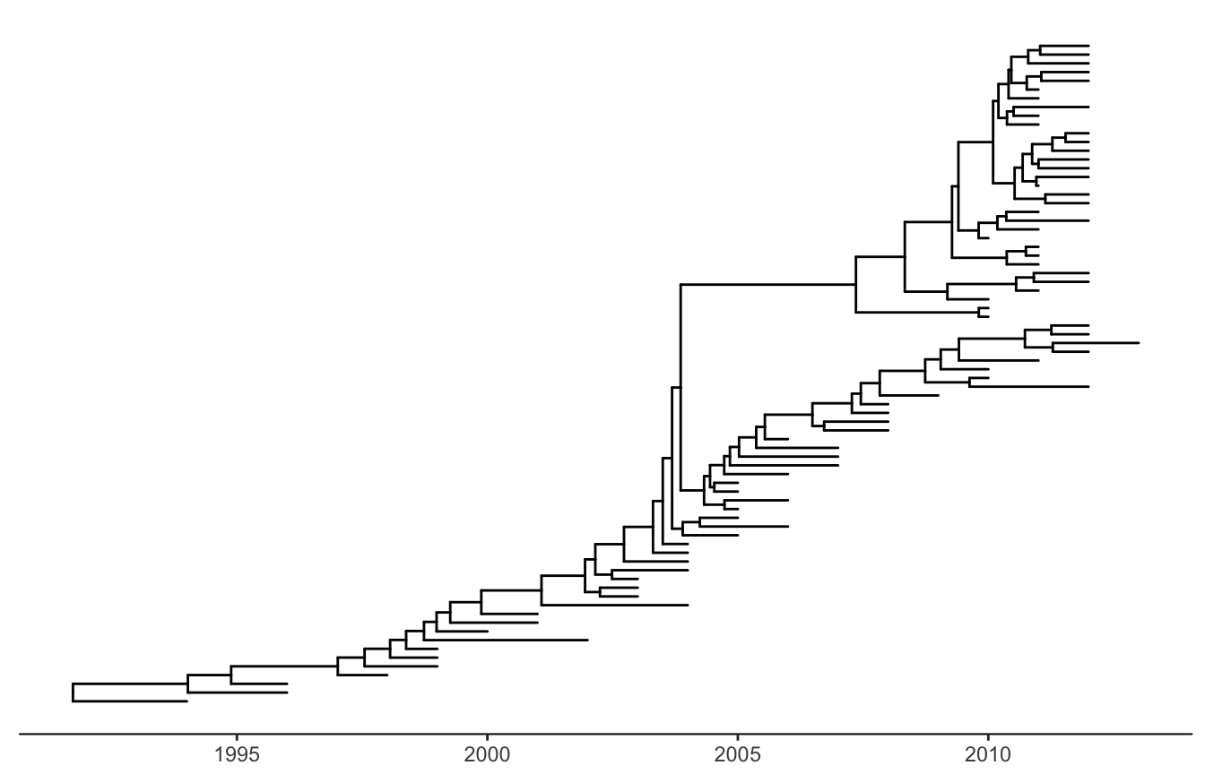
Figure 4.2: Time-scaled layout. The x-axis is the timescale (in units of year). The divergence time was inferred by BEAST using molecular clock model.
Two-dimensional tree layout. A two-dimensional tree is a projection of the phylogenetic tree in a space defined by the associated phenotype (numerical or categorical trait, on the y-axis) and tree branch scale (e.g., evolutionary distance, divergent time, on the x-axis). The phenotype can be a measure of certain biological characteristics of the taxa and hypothetical ancestors in the tree. This is a new layout we proposed in ggtree, which is useful to track the virus phenotypes or other behaviors (y-axis) changing with the virus evolution (x-axis). In fact, the analysis of phenotypes or genotypes over evolutionary time have been widely used for study influenza virus evolution (Neher et al. 2016), though such analysis diagrams are not tree-like, i.e., no connection between data points, unlike our two-dimensional tree layout that connect data points with the corresponding tree branches. Therefore, this new layout we provided will make such data analysis easier and more scalable for large sequence data sets of influenza viruses.
In this example, we used the previous time-scaled tree of H3 human and swine influenza viruses (Figure 4.2; data published in (Liang et al. 2014)) and scaled the y-axis based on the predicted N-linked glycosylation sites (NLG) for each of the taxon and ancestral sequences of hemagglutinin proteins. The NLG sites were predicted using NetNGlyc 1.0 Server8. To scaled the y-axis, the parameter yscale in the ggtree() function is set to a numerical or categorical variable. If yscale is a categorical variable as in this example, users should specify how the categories are to be mapped to numerical values via the yscale_mapping variables.
NAG_file <- system.file("examples/NAG_inHA1.txt", package="ggtree")

NAG.df <- read.table(NAG_file, sep="\t", header=FALSE,
                     stringsAsFactors = FALSE)
NAG <- NAG.df[,2]
names(NAG) <- NAG.df[,1]

## separate the tree by host species
tip <- get.tree(beast_tree)$tip.label
beast_tree <- groupOTU(beast_tree, tip[grep("Swine", tip)],
                       group_name = "host")

p <- ggtree(beast_tree, aes(color=host), mrsd="2013-01-01",
            yscale = "label", yscale_mapping = NAG) +
  theme_classic() + theme(legend.position='none') +
  scale_color_manual(values=c("blue", "red"),
                     labels=c("human", "swine")) +
  ylab("Number of predicted N-linked glycoslyation sites")

## (optional) add more annotations to help interpretation
p + geom_nodepoint(color="grey", size=3, alpha=.8) +
  geom_rootpoint(color="black", size=3) +
  geom_tippoint(size=3, alpha=.5) +
  annotate("point", 1992, 5.6, size=3, color="black") +
  annotate("point", 1992, 5.4, size=3, color="grey") +
  annotate("point", 1991.6, 5.2, size=3, color="blue") +
  annotate("point", 1992, 5.2, size=3, color="red") +
  annotate("text", 1992.3, 5.6, hjust=0, size=4, label="Root node") +
  annotate("text", 1992.3, 5.4, hjust=0, size=4,
           label="Internal nodes") +
  annotate("text", 1992.3, 5.2, hjust=0, size=4,
           label="Tip nodes (blue: human; red: swine)")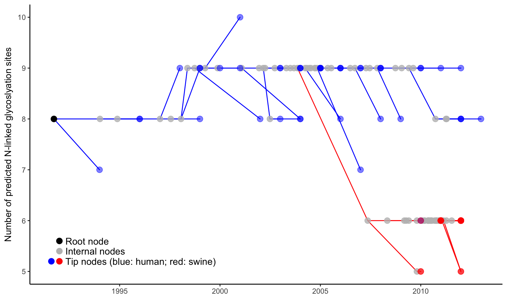
Figure 4.3: Two-dimensional tree layout. The trunk and other branches highlighted in red (for swine) and blue (for human). The x-axis is scaled to the branch length (in units of year) of the time-scaled tree. The y-axis is scaled to the node attribute variable, in this case the number of predicted N-linked glycosylation site (NLG) on the hemagglutinin protein. Colored circles indicate the different types of tree nodes. Note that nodes assigned the same x- (temporal) and y- (NLG) coordinates are superimposed in this representation and appear as one node, which is shaded based on the colors of all the nodes at that point.
As shown in Figure 4.3, two-dimensional tree good at visualizing the change of phenotype over the evolution in the phylogenetic tree. In this example, it is shown that H3 gene of human influenza A virus maintained high level of N-linked glycosylation sites (n=8 to 9) over last two decades and dropped significantly to 5 or 6 in a separate viral lineage transmitted to swine populations and established there. It was indeed hypothesized that the human influenza virus with high level of glycosylation on the viral hemagglutinin protein provides better shielding effect to protect the antigenic sites from exposure to the herd immunity, and thus has selective advantage in human populations that maintain high level of herd immunity against the circulating human influenza virus strains. For the viral lineage that newly jumped across the species barrier and transmitted to swine population, the shielding effect of the high-level surface glycan oppositely impose selective disadvantage because the receptor-binding domain may also be shielded which greatly affect the viral fitness of the lineage that newly adapted to a new host species.
4.3.3 Annotation layers
The ggtree is designed for more general purpose or specific type of tree visualization and annotation. It supports grammar of graphics implemented in ggplot2 and users can freely visualize/annotate a tree by combining several annotation layers.
library(ggtree)
treetext = "(((ADH2:0.1[&&NHX:S=human], ADH1:0.11[&&NHX:S=human]):
0.05 [&&NHX:S=primates:D=Y:B=100],ADHY:
0.1[&&NHX:S=nematode],ADHX:0.12 [&&NHX:S=insect]):
0.1[&&NHX:S=metazoa:D=N],(ADH4:0.09[&&NHX:S=yeast],
ADH3:0.13[&&NHX:S=yeast], ADH2:0.12[&&NHX:S=yeast],
ADH1:0.11[&&NHX:S=yeast]):0.1[&&NHX:S=Fungi])[&&NHX:D=N];"
tree <- read.nhx(textConnection(treetext))
ggtree(tree) + geom_tiplab() +
  geom_label(aes(x=branch, label=S), fill='lightgreen') +
  geom_label(aes(label=D), fill='steelblue') +
  geom_text(aes(label=B), hjust=-.5)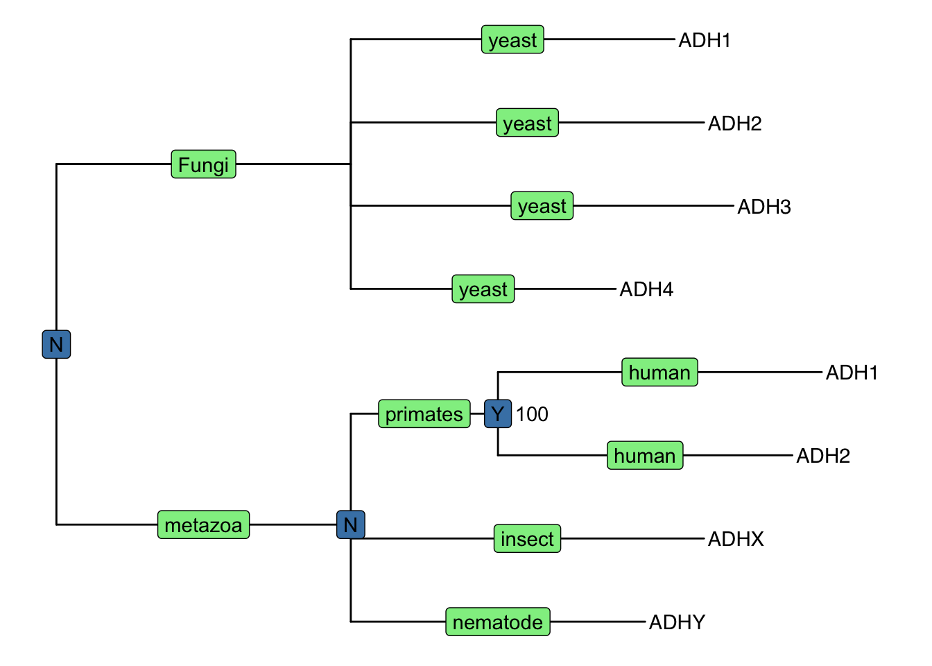
Figure 4.4: Annotating tree using grammar of graphics. The NHX tree was annotated using grammar of graphic syntax by combining different layers using + operator. Species information were labelled on the middle of the branches, Duplication events were shown on most recent common ancestor and clade bootstrap value were dispalyed near to it.
Here, as an example, we visualized the tree with several layers to display annotation stored in NHX tags, including a layer of geom_tiplab to display tip labels (gene name in this case), a layer using geom_label to show species information (S tag) colored by lightgreen, a layer of duplication event information (D tag) colored by steelblue and another layer using geom_text to show bootstrap value (B tag).
Layers defined in ggplot2 can be applied to ggtree directly as demonstrated in Figure 4.4 of using geom_label and geom_text. But ggplot2 does not provide graphic layers that are specific designed for phylogenetic tree annotation. For instance, layers for tip labels, tree branch scale legend, highlight or labeling clade are all unavailable. To make tree annotation more flexible, a number of layers have been implemented in ggtree (Table 4.1), enabling different ways of annotation on various parts/components of a phylogenetic tree.
| Layer | Description |
|---|---|
| geom_balance | highlights the two direct descendant clades of an internal node |
| geom_cladelabel | annotate a clade with bar and text label |
| geom_hilight | highlight a clade with rectangle |
| geom_label2 | modified version of geom_label, with subsetting supported |
| geom_nodepoint | annotate internal nodes with symbolic points |
| geom_point2 | modified version of geom_point, with subsetting supported |
| geom_range | bar layer to present uncertainty of evolutionary inference |
| geom_rootpoint | annotate root node with symbolic point |
| geom_segment2 | modified version of geom_segment, with subsetting supported |
| geom_strip | annotate associated taxa with bar and (optional) text label |
| geom_taxalink | associate two related taxa by linking them with a curve |
| geom_text2 | modified version of geom_text, with subsetting supported |
| geom_tiplab | layer of tip labels |
| geom_tiplab2 | layer of tip labels for circular layout |
| geom_tippoint | annotate external nodes with symbolic points |
| geom_tree | tree structure layer, with multiple layout supported |
| geom_treescale | tree branch scale legend |
4.3.4 Tree manipulation
The ggtree supports many ways of manipulating the tree visually, including viewing selected clade to explore large tree (Figure 4.5), taxa clustering (Figure 4.8), rotating clade or tree (Figure 4.9B and 4.11), zoom out or collapsing clades (Figure 4.6A and 4.7), etc.. Details tree manipulation functions are summarized in Table 4.2.
| Function | Descriptiotn |
|---|---|
| collapse | collapse a selecting clade |
| expand | expand collapsed clade |
| flip | exchange position of 2 clades that share a parent node |
| groupClade | grouping clades |
| groupOTU | grouping OTUs by tracing back to most recent common ancestor |
| identify | interactive tree manipulation |
| rotate | rotating a selected clade by 180 degree |
| rotate_tree | rotating circular layout tree by specific angle |
| scaleClade | zoom in or zoom out selecting clade |
| open_tree | convert a tree to fan layout by specific open angle |
A clade is a monophyletic group that contains a single ancestor and all of its descendants. We can visualize a specific selected clade via the viewClade function as demonstrated in Figure 4.5B. Another similar function is gzoom which plots the tree with selected clade side by side. These two functions are developed to explore large tree.
library(ggtree)
nwk <- system.file("extdata", "sample.nwk", package="treeio")
tree <- read.tree(nwk)
p <- ggtree(tree) + geom_tiplab()
viewClade(p, MRCA(p, tip=c("I", "L")))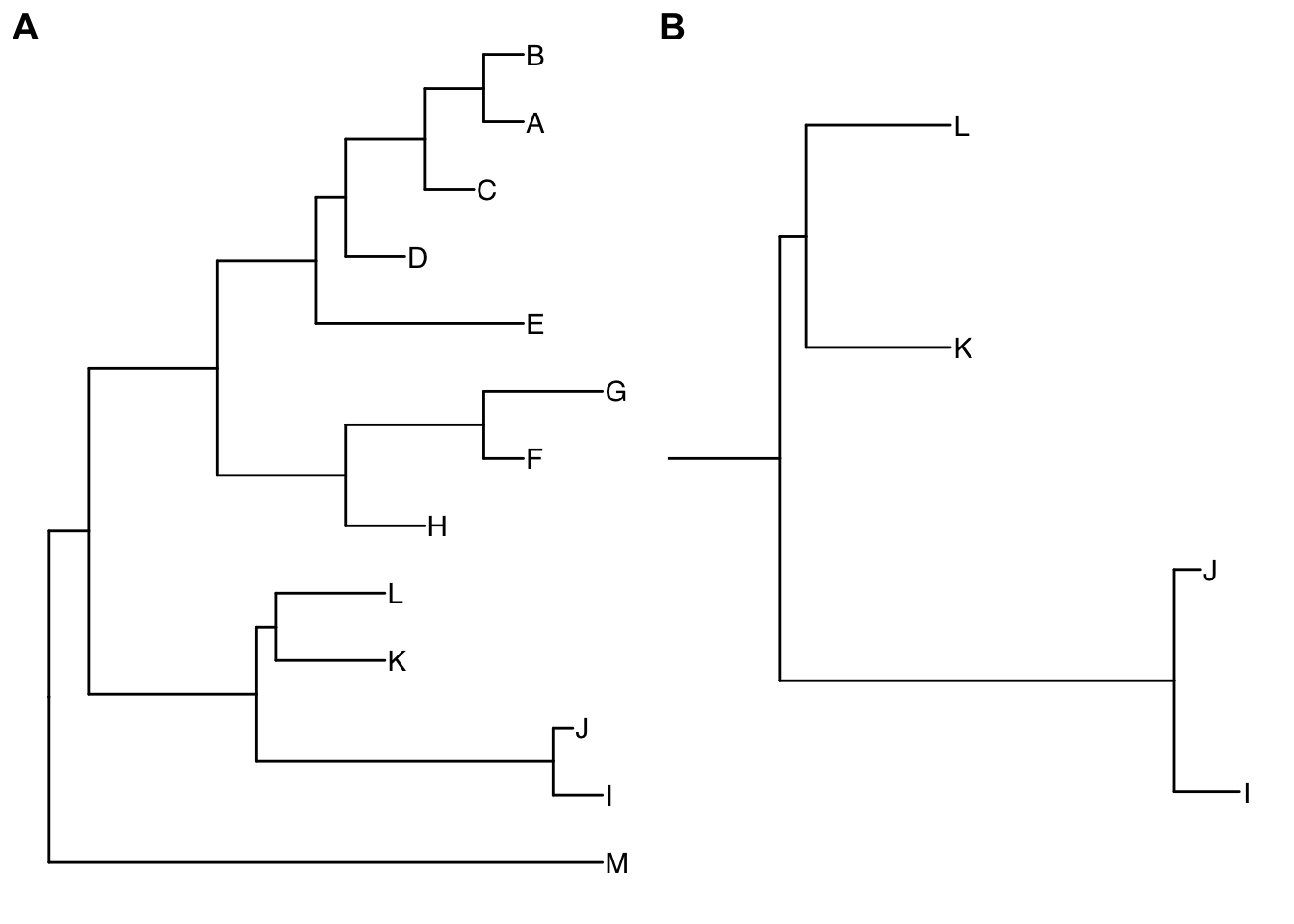
Figure 4.5: Viewing a selected clade of a tree. An example tree used to demonstrate how ggtree support exploring or manipulating phylogenetic tree visually (A). The ggtree supports visualizing selected clade (B). A clade can be selected by specifying a node number or determined by most recent common ancestor of selected tips.
It is a common practice to prune or collapse clades so that certain aspects of a tree can be emphasized. The ggtree supports collapsing selected clades using the collapse function as shown in Figure 4.6A.
p2 <- p %>% collapse(node=21) +
  geom_point2(aes(subset=(node==21)), shape=21, size=5, fill='green')
p2 <- collapse(p2, node=23) +
  geom_point2(aes(subset=(node==23)), shape=23, size=5, fill='red')
print(p2)
expand(p2, node=23) %>% expand(node=21)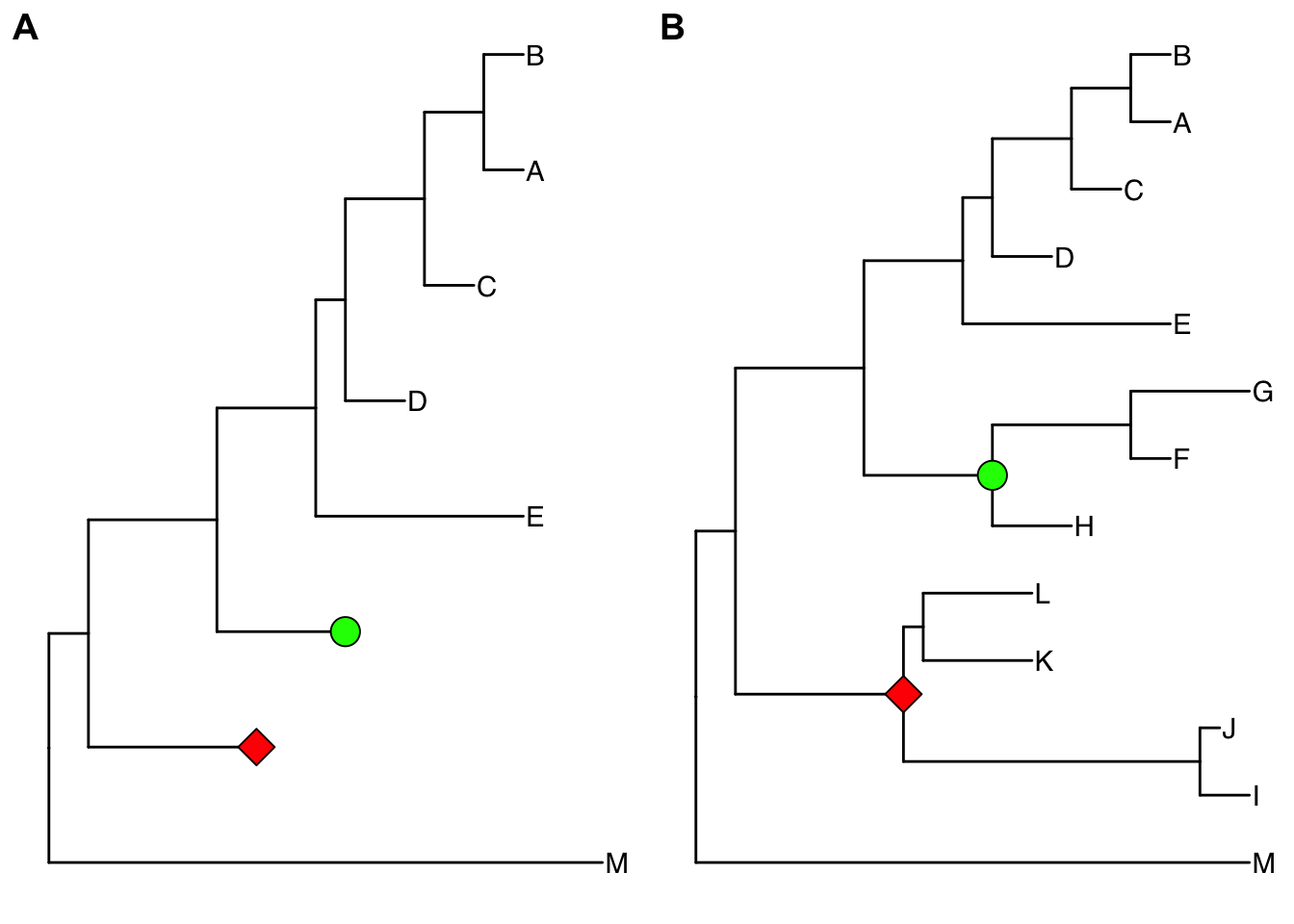
Figure 4.6: Collapsing selected clades and expanding collapsed clades. Clades can be selected to collapse (A) and the collapsed clades can be expanded back (B) if necessary as ggtree stored all information of species relationships. Green and red symbols were displayed on the tree to indicate the collapsed clades.
Here two clades were collapsed and labelled by green circle and red square symbolic points. Collapsing is a common strategy to collapse clades that are too large for displaying in full or are not primary interest of the study. In ggtree, we can expand (i.e., uncollapse) the collapsed branches back with expand function to show details of species relationships as demonstrated in Figure 4.6B.
The ggtree provides another option to zoom out (or compress) these clades via the scaleClade function. In this way, we retain the topology and branch lengths of compressed clades. This helps to save the space to highlight those clades of primary interest to the study.
tree2 <- groupClade(tree, c(17, 21))
p <- ggtree(tree2, aes(color=group)) +
  scale_color_manual(values=c("black", "firebrick", "steelblue"))
scaleClade(p, node=17, scale=.1) 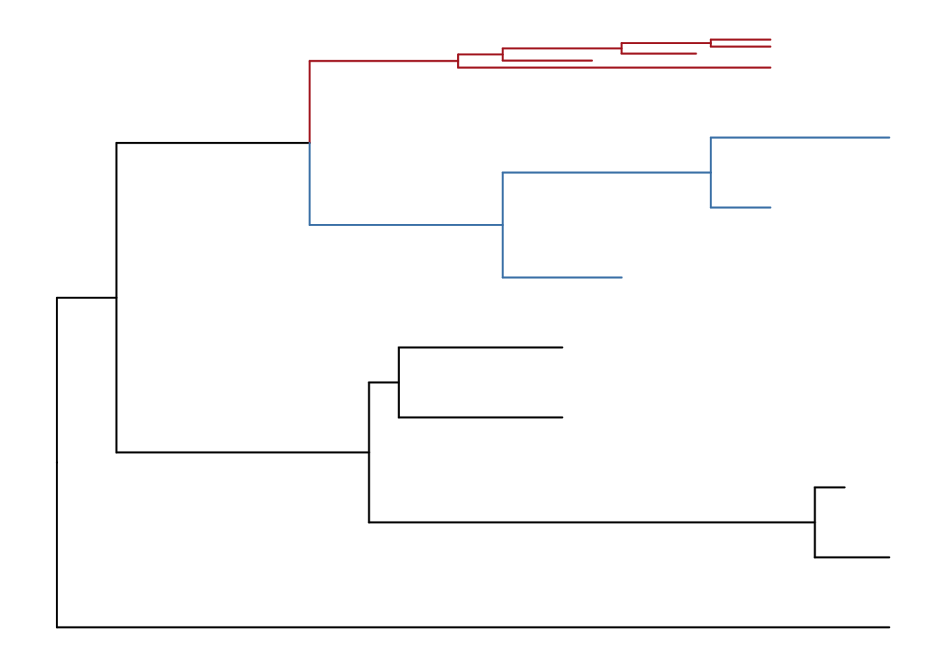
Figure 4.7: Scaling selected clade. Clades can be zoom in (if scale > 1) to highlight or zoom out to save space.
If users want to emphasize important clades, they can use scaleClade function with scale parameter larger than 1. Then the selected clade will be zoomed in. Users can also use groupClade to select clades and color them with different colors as shown in Figure 4.7.
Although groupClade works fine with clade (monophyletic), related taxa are not necessarily within a clade, they can be polyphyletic or paraphyletic. The ggtree implemented groupOTU to work with polyphyletic and paraphyletic. It accepts a vector of OTUs (taxa name) or a list of OTUs and will trace back from OTUs to their most recent common ancestor (MRCA) and cluster them together as demonstrated in Figure 4.8.
tree2 <- groupOTU(tree, focus=c("D", "E", "F", "G"))
ggtree(tree2, aes(color=group)) + geom_tiplab()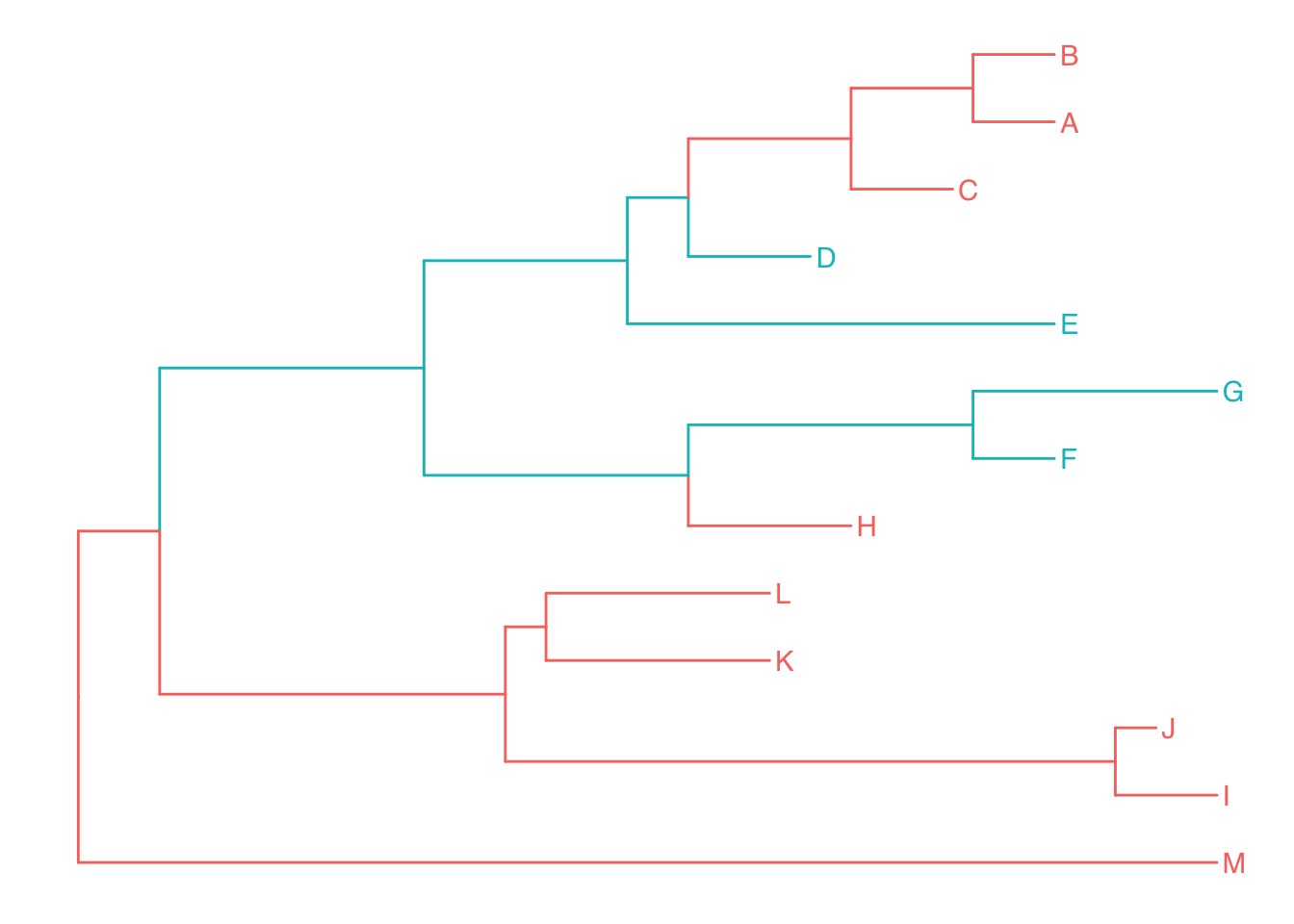
Figure 4.8: Grouping OTUs. OTU clustering based on their relationships. Selected OTUs and their ancestors upto MRCA will be clustered together.
To facilitate exploring the tree structure, ggtree supports rotating selected clade by 180 degree using the rotate function (Figure 4.9B). Position of immediate descendant clades of internal node can be exchanged via flip function (Figure 4.9C).
p1 <- p + geom_point2(aes(subset=node==16), color='darkgreen', size=5)
p2 <- rotate(p1, 17) %>% rotate(21)
flip(p2, 17, 21)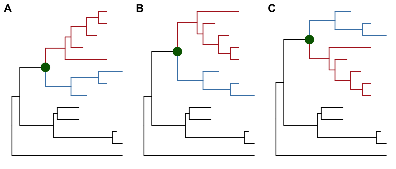
Figure 4.9: Exploring tree structure. A clade (indicated by darkgreen circle) in a tree (A) can be rotated by 180° (B) and the positions of its immediate descedant clades (colored by blue and red) can be exchanged (C).
Most of the tree manipulation functions are working on clades, while ggtree also provides functions to manipulate a tree, including open_tree to transform a tree in either rectangular or circular layout to fan layout, and rotate_tree function to rotate a tree for specific angle in both circular or fan layouts, as demonstrated in Figure 4.10 and 4.11.
p3 <- open_tree(p, 180) + geom_tiplab2()
print(p3)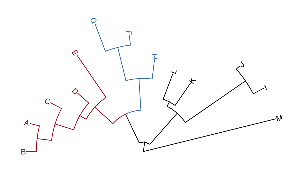
Figure 4.10: Transforming a tree to fan layout. A tree can be transformed to fan layout by open_tree with specific angle parameter.
rotate_tree(p3, 180)
Figure 4.11: Rotating tree. A circular/fan layout tree can be rotated by any specific angle.
4.3.5 Tree annotation using data from evolutionary analysis software
Chapter 2 has introduced using treeio packages to parse different tree formats and commonly used software outputs to obtain phylogeny-associated data. These imported data as S4 objects can be visualized directly using ggtree. Figure 4.4 demonstrates a tree annotated using the information (species classification, duplication event and bootstrap value) stored in NHX file. PHYLODOG and RevBayes output NHX files that can be parsed by treeio and visualized by ggtree with annotation using their inference data.
Furthermore, the evolutionary data from the inference of BEAST, MrBayes and RevBayes, dN/dS values inferred by CodeML, ancestral sequences inferred by HyPhy, CodeML or BaseML and short read placement by EPA and pplacer can be used to annotate the tree directly.
file <- system.file("extdata/BEAST", "beast_mcc.tree",
                    package="treeio")
beast <- read.beast(file)
ggtree(beast) +
  geom_tiplab(align=TRUE, linetype='dashed', linesize=.3) +
  geom_range("length_0.95_HPD", color='red', size=2, alpha=.5) +
  geom_text2(aes(label=round(as.numeric(posterior), 2),
                 subset=as.numeric(posterior)> 0.9,
x=branch), vjust=0) 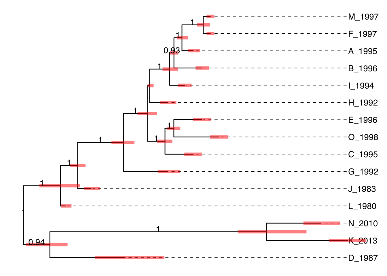
Figure 4.12: Annotating BEAST tree with length_95%_HPD and posterior. Branch length credible intervals (95% HPD) were displayed as red horizontal bars and clade posterior values were shown on the middle of branches.
In Figure 4.12, the tree was visualized and annotated with posterior > 0.9 and demonstrated length uncertainty (95% Highest Posterior Density (HPD) interval).
Ancestral sequences inferred by HyPhy can be parsed using treeio, whereas the substitutions along each tree branch was automatically computed and stored inside the phylogenetic tree object (i.e., S4 object). The ggtree can utilize this information in the object to annotate the tree, as demonstrated in Figure 4.13.
nwk <- system.file("extdata/HYPHY", "labelledtree.tree",
                   package="treeio")
ancseq <- system.file("extdata/HYPHY", "ancseq.nex",
                      package="treeio")
tipfas <- system.file("extdata", "pa.fas", package="treeio")
hy <- read.hyphy(nwk, ancseq, tipfas)
ggtree(hy) +
  geom_text(aes(x=branch, label=AA_subs), size=2,
            vjust=-.3, color="firebrick")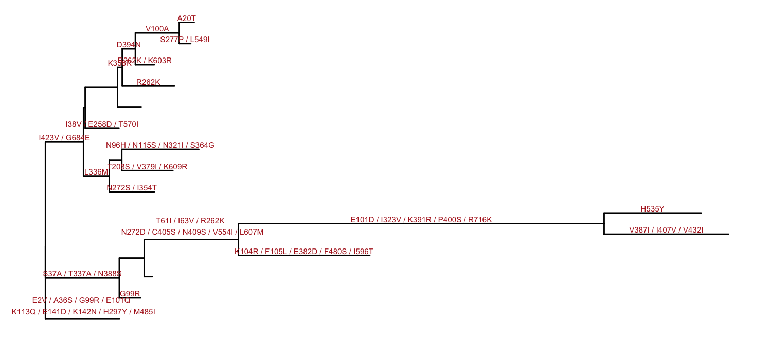
Figure 4.13: Annotating tree with amino acid substitution determined by ancestral sequences inferred by HYPHY. Amino acid substitutions were displayed on the middle of branches.
PAML’s BaseML and CodeML can be also used to infer ancestral sequences, whereas CodeML can infer selection pressure. After parsing this information using treeio, ggtree can integrate this information into the same tree structure and used for annotation as illustrated in Figure 4.14.
rstfile <- system.file("extdata/PAML_Codeml", "rst",
                       package="treeio")
mlcfile <- system.file("extdata/PAML_Codeml", "mlc",
                       package="treeio")
ml <- read.codeml(rstfile, mlcfile)
ggtree(ml, aes(color=dN_vs_dS), branch.length='dN_vs_dS') +
  scale_color_continuous(name='dN/dS', limits=c(0, 1.5),
                         oob=scales::squish,
                         low='darkgreen', high='red') +
  geom_text(aes(x=branch, label=joint_AA_subs),
            vjust=-.5, color='steelblue', size=2) +
  theme_tree2(legend.position=c(.9, .3))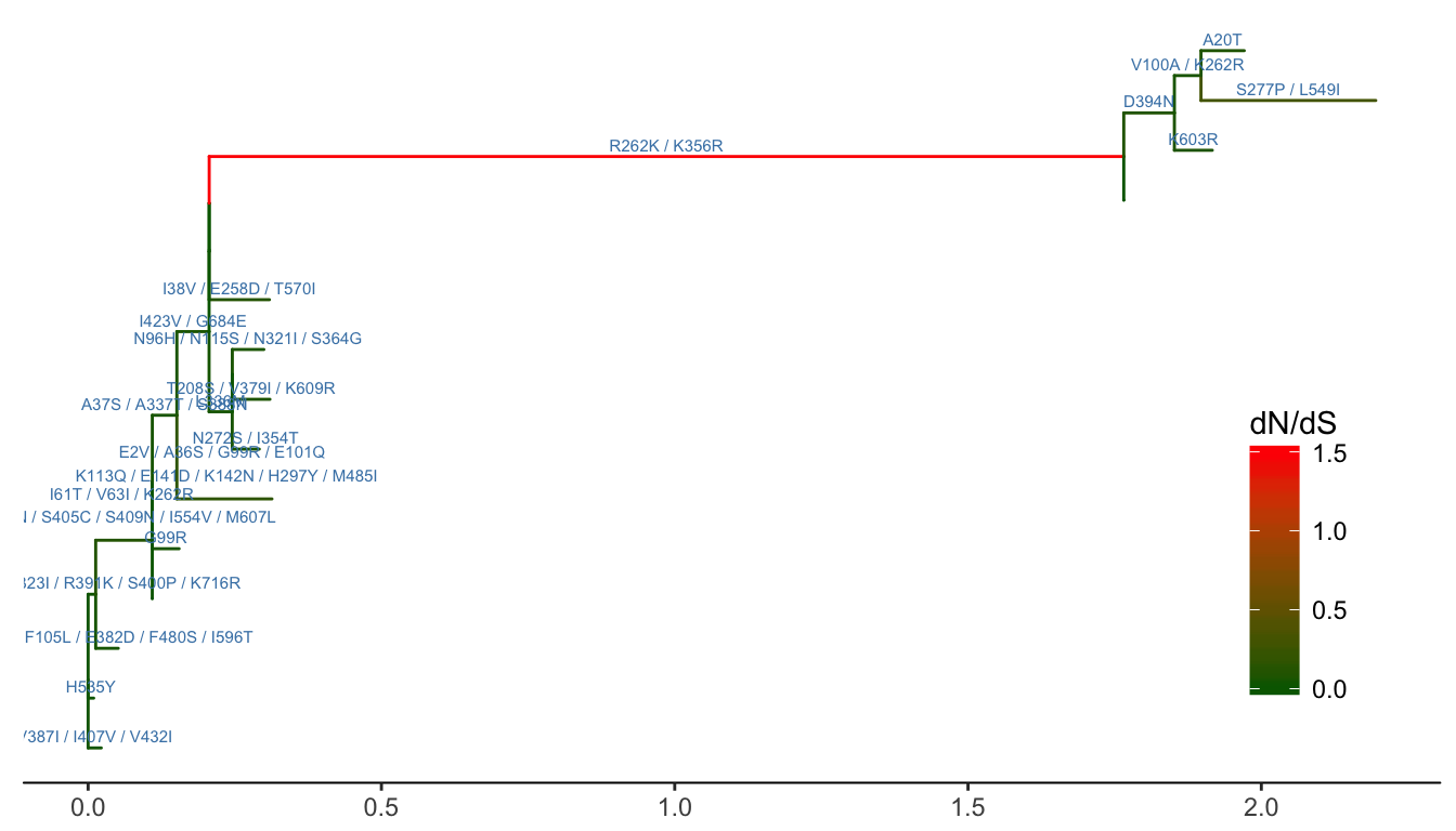
Figure 4.14: Annotating tree with animo acid substitution and dN/dS inferred by CodeML. Branches were rescaled and colored by dN/dS values and amino acid substitutions were displayed on the middle of branches.
For more details and examples of annotating tree with evolutionary data inferred by different software packages can be referred to the online vignettes9.
4.3.6 Tree annotation based on tree classes defined in other R packages
The ggtree plays a unique role in R ecosystem to facilitate phylogenetic analysis. It serves as a generic tools for tree visualization and annotation with different associated data from various sources. Most of the phylogenetic tree classes defined in R community are supported, including obkData, phyloseq, phylo, multiPhylo, phylo4 and phylo4d. Such that ggtree can be easily integrated into their analysis/packages. For instance, phyloseq users will find ggtree useful for visualizing microbiome data and for further annotations, since ggtree supports high-level of annotation using grammar of graphics and some of its features are not available in phyloseq. Here, examples of using ggtree to annotate obkData and phyloseq tree objects are demonstrated. There example data can be found in vignettes of OutbreakTools (Jombart et al. 2014) and phyloseq (McMurdie and Holmes 2013) packages.
The okbData is defined to store incidence-based outbreak data, including meta data of sampling and information of infected individuals such as age and onset of symptoms. The ggtree supports parsing this information which was used to annotate the tree as shown in Figure 4.15.
library(OutbreakTools)
data(FluH1N1pdm2009)
attach(FluH1N1pdm2009)

x <- new("obkData",
         individuals = individuals,
         dna = dna,
         dna.individualID = samples$individualID,
         dna.date = samples$date,
         trees = FluH1N1pdm2009$trees)
ggtree(x, mrsd="2009-09-30", as.Date=TRUE, right=TRUE) +
    geom_tippoint(aes(color=location), size=3, alpha=.75) +
    scale_color_brewer("location", palette="Spectral") +
    theme_tree2(legend.position='right')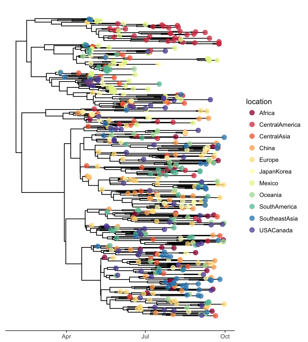
Figure 4.15: Visualizing obkData tree object. x-axis was scaled by timeline of the outbreak and tips were colored by location of different individuals.
The phyloseq class that defined in the phyloseq package was designed for storing microbiome data, including phylogenetic tree, associated sample data and taxonomy assignment. It can import data from popular pipelines, such as QIIME (Kuczynski et al. 2011), mothur (Schloss et al. 2009), DADA2 (Callahan et al. 2016) and PyroTagger (Kunin and Hugenholtz 2010), etc.. The ggtree supports visualizing the phylogenetic tree stored in phyloseq object and related data can be used to annotate the tree as demonstrated in Figure 4.16.
library(phyloseq)
library(ggjoy)
library(dplyr)
library(ggtree)

data("GlobalPatterns")
GP <- GlobalPatterns
GP <- prune_taxa(taxa_sums(GP) > 600, GP)
sample_data(GP)$human <- get_variable(GP, "SampleType") %in%
  c("Feces", "Skin")

mergedGP <- merge_samples(GP, "SampleType")
mergedGP <- rarefy_even_depth(mergedGP,rngseed=394582)
mergedGP <- tax_glom(mergedGP,"Order")

melt_simple <- psmelt(mergedGP) %>%
  filter(Abundance < 120) %>%
  select(OTU, val=Abundance)

p <- ggtree(mergedGP) +
  geom_tippoint(aes(color=Phylum), size=1.5)

facet_plot(p, panel="Abundance", data=melt_simple,
           geom_joy, mapping = aes(x=val,group=label,
                                        fill=Phylum),
           color='grey80', lwd=.3)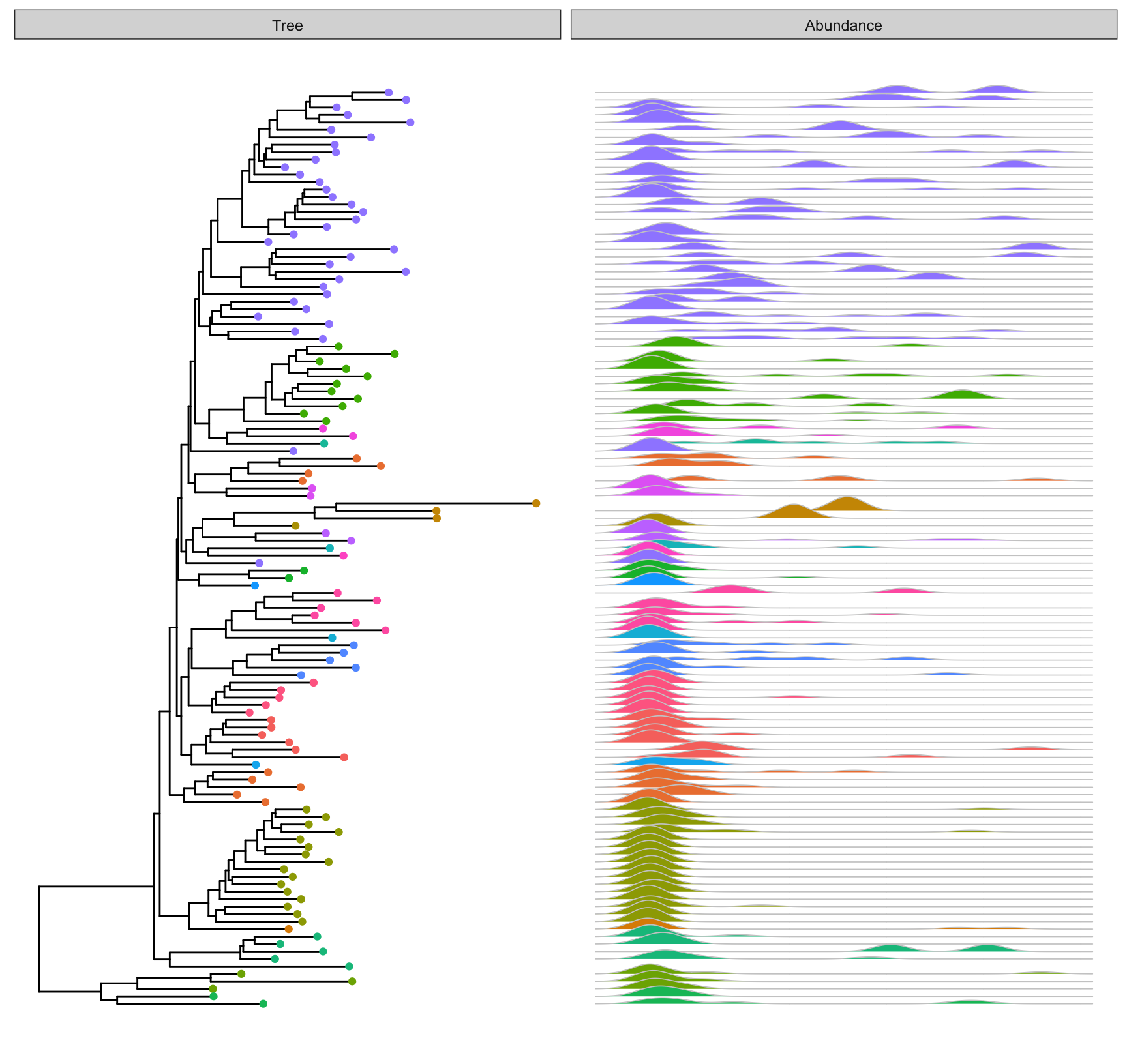
Figure 4.16: Visualizing phyloseq tree object. Tips were colored by Phylum and corresponding abundance across different samples were visualized as joyplots and sorted according to the tree structure.
4.3.7 Advanced annotation on the phylogenetic tree
The ggtree supports grammar of graphics that implemented in ggplot2 package and provides several layers and functions to facilitate phylogenetic visualization and annotation. These layers and functions are not designed for specific tasks, they are building blocks that can be freely combined together to produce complex tree figure. Previous sessions have introduced some important functions of ggtree. In this session, three examples were presented to demonstrate using various ggtree functions together to construct a complex tree figure with annotations by associated data and inference results from different analysis programs.
4.3.7.1 Example 1: plot curated gene information as heatmap
This example introduces annotating a tree with various sources of data (e.g., location, sampling year, curated genotype information, etc.).
## use the following command to get the data from Holt Lab
## git clong https://github.com/katholt/plotTree.git

setwd("plotTree/tree_example_april2015/")

info <- read.csv("info.csv")
tree <- read.tree("tree.nwk")
cols <- c(HCMC='black', Hue='purple2', KH='skyblue2')

p <- ggtree(tree, layout='circular') %<+% info +
  geom_tippoint(aes(color=location)) +
  scale_color_manual(values=cols) +
  geom_tiplab2(aes(label=name), align=T, linetype=NA,
              size=2, offset=4, hjust=0.5) +
  geom_tiplab2(aes(label=year), align=T, linetype=NA,
              size=2, offset=8, hjust=0.5)
The tree was visualized in circular layout and attached with the strain sampling location information. A geom_tippoint layer added circular symbolic points to tree tips and colored them by their locations. Two geom_tiplab2 were added to display taxon names and sampling years.
heatmapData=read.csv("res_genes.csv", row.names=1)
rn <- rownames(heatmapData)
heatmapData <- as.data.frame(sapply(heatmapData, as.character))
rownames(heatmapData) <- rn

heatmap.colours <- c("white","grey","seagreen3","darkgreen",
                    "green","brown","tan","red","orange",
                    "pink","magenta","purple","blue","skyblue3",
                    "blue","skyblue2")
names(heatmap.colours) <- 0:15

gheatmap(p, heatmapData, offset = 10, color=NULL,
         colnames_position="top",
         colnames_angle=90, colnames_offset_y = 1,
         hjust=0, font.size=2) +
  scale_fill_manual(values=heatmap.colours, breaks=0:15)
The curated gene information was further loaded and plotted as a heatmap using gheatmap function with customized colors. The final figure was demonstrated in Figure 4.17.
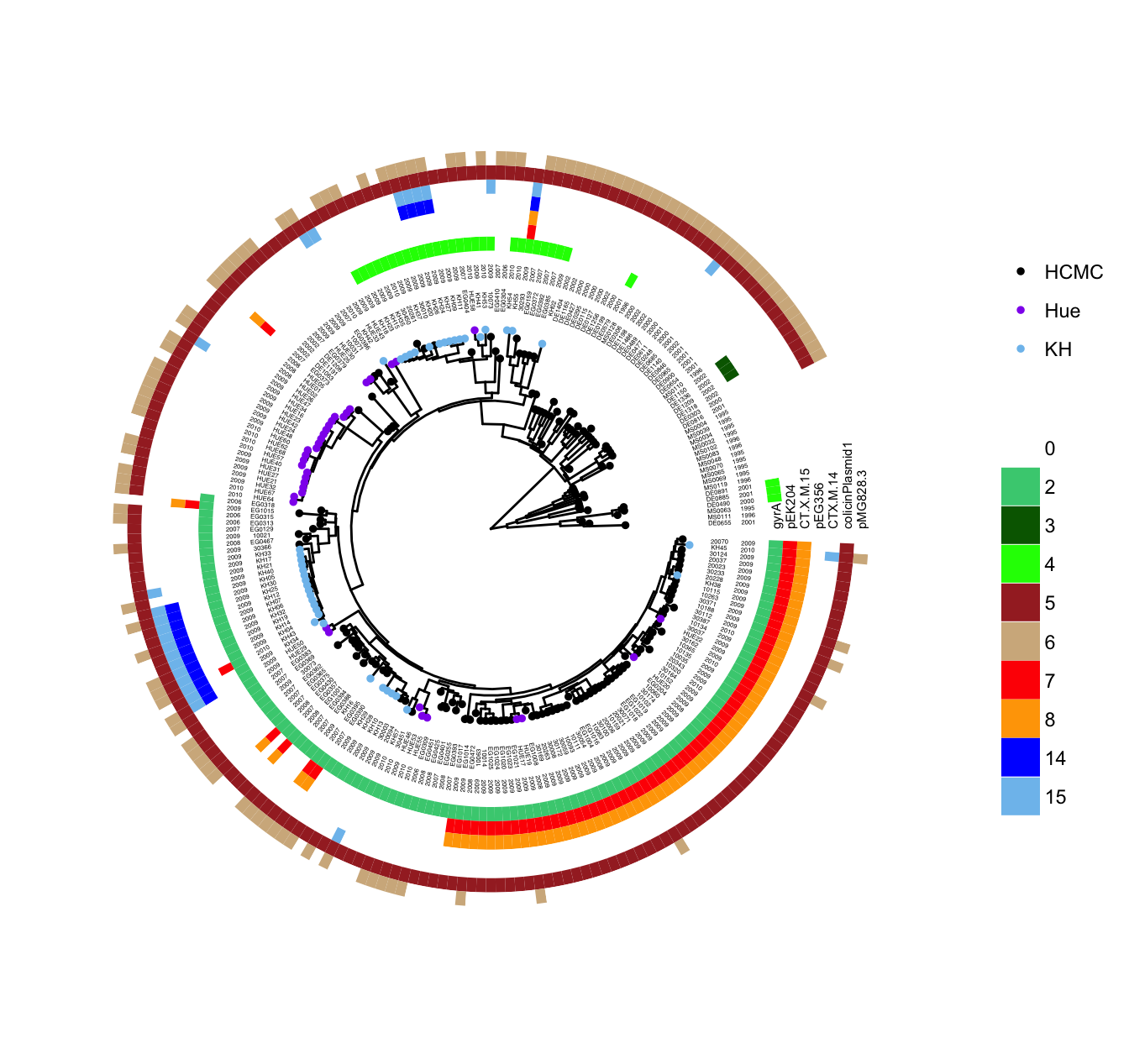
Figure 4.17: Example of annotating a tree with diverse associated data. Circle symbols are colored by strain sampling location. Taxa names and sampling years are aligned to the tips. Curated gene information were visualized as a heatmap (colored boxed on the outer circles).
4.3.7.2 Example 2: complex tree annotations
The ggtree allows various evidences inferred by different software to be integrated, compared and visualized on a same tree topology. Data from external files can be further integrated for analysis and visualization. This example introduces complex tree annotations with evolutionary data inferred by different software (BEAST and CodeML in this example) and other associated data (e.g., genotype table).
library(treeio)
library(ggtree)

beast_file <- system.file("examples/MCC_FluA_H3.tree",
                          package="ggtree")
rst_file <- system.file("examples/rst", package="ggtree")
mlc_file <- system.file("examples/mlc", package="ggtree")

beast_tree <- read.beast(beast_file)
codeml_tree <- read.codeml(rst_file, mlc_file)
merged_tree <- merge_tree(beast_tree, codeml_tree)

cols <- scale_color(merged_tree, "dN_vs_dS",
                    low="#0072B2", high="#D55E00",
                    interval=seq(0, 1.5, length.out=100))
p <- ggtree(merged_tree, size=.8, mrsd="2013-01-01",
            ndigits = 2, color=cols)
p <- add_colorbar(p, cols, font.size=3)

p <- p + geom_text(aes(label=posterior), color="darkgreen",
                   vjust=-.1, hjust=-.03, size=1.8)
First of all, BEAST and CodeML outputs were parsed, and the two trees with the associated data were merged into one. After merging, all statistical data inferred by these software packages, including divergence time and dN/dS will be incorporated into the merged_tree object. The tree was first visualized in time-scale and its branches were colored with dN/dS, and annotated the tree with posterior clade probabilities.
site_file <- system.file("examples/sites.txt", package="ggtree")
site <- read.table(site_file)[,1]
tree <- mask(merged_tree, "joint_AA_subs", site, mask_site = FALSE)
p <- p + geom_text(aes(x=branch, label=joint_AA_subs),
                   vjust=-.03, size=1.8)
The tree branches were further annotated with amino acid substitutions pre-computed from taxon sequences and the ancestral sequences imported from CodeML.
tip <- get.tree(merged_tree)$tip.label
host <- rep("Human", length(tip))
host[grep("Swine", tip)] <- "Swine"
host.df <- data.frame(taxa=tip, host=factor(host))

p <- p %<+% host.df + geom_tippoint(aes(color=host), size=2) +
  geom_tiplab(aes(color=host), align=TRUE, size=3, linesize=.3) +
  scale_color_manual(values = c("#377EB8", "#E41A1C"), guide='none')
Symbolic points were added to tree tips with different colors to differentiate host species of the influenza virus samples (blue for human and red for swine).
genotype_file <- system.file("examples/Genotype.txt", package="ggtree")
genotype <- read.table(genotype_file, sep="\t", stringsAsFactor=F)
colnames(genotype) <- sub("\\.", "", colnames(genotype))
genotype[genotype == "trig"] <- "TRIG"
genotype[genotype == "pdm"] <- "Pdm/09"

p <- gheatmap(p, genotype, width=.4, offset=7, colnames=F) %>%
  scale_x_ggtree
p + scale_fill_brewer(palette="Set2") + theme_tree2() +
  scale_y_continuous(expand=c(0, 0.6)) + xlab("Time") +
  theme(legend.text=element_text(size=8),
        legend.key.height=unit(.5, "cm"),
        legend.key.width=unit(.4, "cm"),
        legend.position=c(.13, y=.945),
        axis.text.x=element_text(size=10),
        axis.title.x = element_text(size=12))
Finally, a genotype table (imported from external file) was plotted as a heatmap and aligned to the tree according to the tree structure as shown in Figure 4.18.
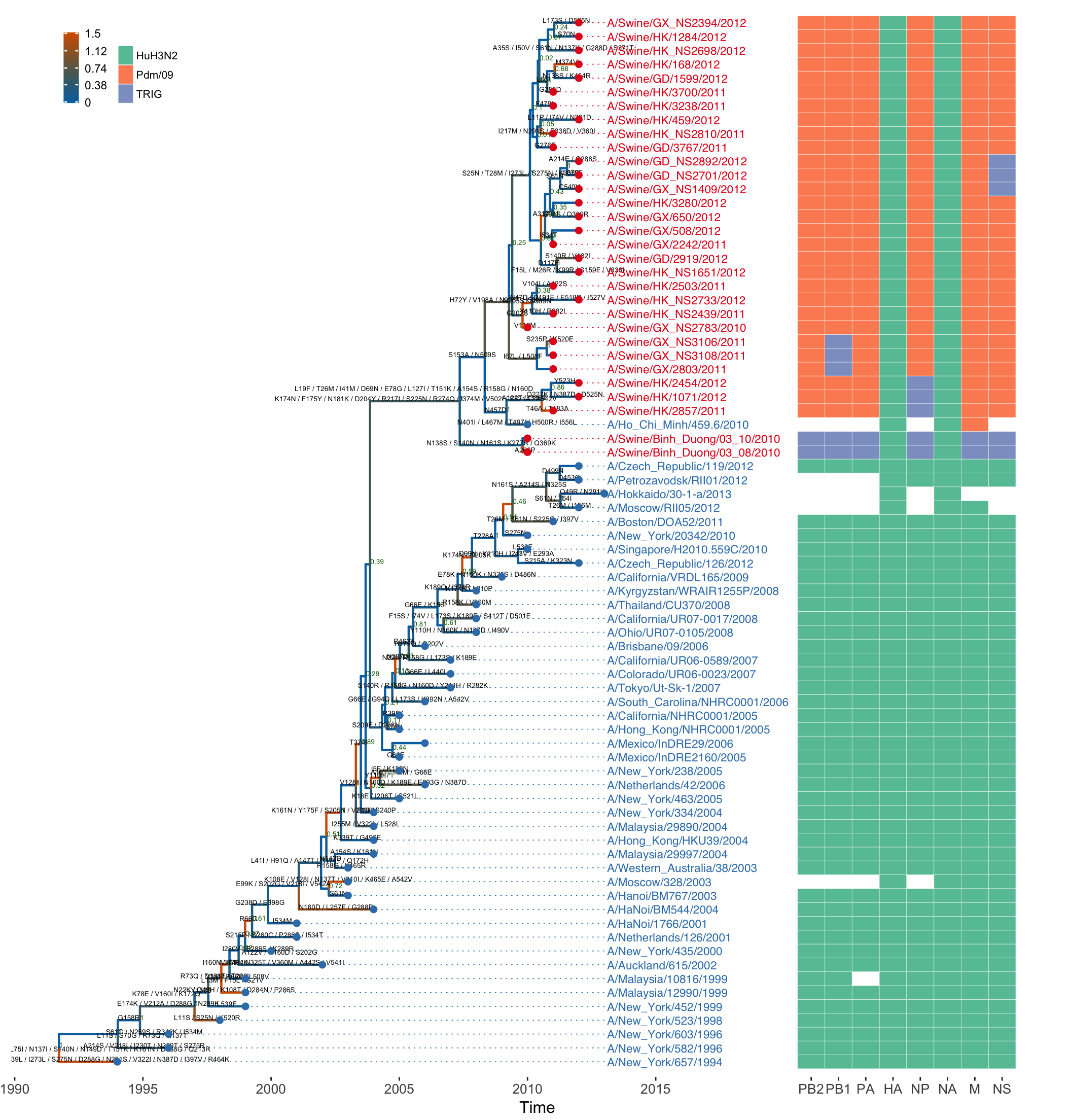
Figure 4.18: Example of annotating a tree with evolutionary evidences inferred by different software. The x-axis is the time scale (in units of year) inferred by BEAST. The tree branches are colored by their dN/dS values (as in the left scale at the top) inferred by CodeML, and the internal node labels show the posteria probabilities inferred by BEAST. Tip labels (taxon names) and circles are colored by species (human in blue and swine in red). The genotype, which is shown as an array of colored boxes on the right, is composed of the lineages (either HuH3N2, Pdm/09 or TRIG, colored as in the right legend at the top) of the eight genome segments of the virus. Any missing segment sequences are shown as empty boxes.
4.3.7.3 Example 3: Integrating ggtree in analysis pipeline/workflow
In the first example, a tree figure was annotated with external data, whereas second example introduced more complex annotations with evolutionary data inferred by different software and other associated data. This example will demonstrate integrating ggtree to an analysis pipeline that start from nucleotide sequence, building a tree, using R package to inferred ancestral sequences and states, then using ggtree to integrate these inferences to visualize and interpret results to help identify evolutionary patterns.
In this example, we collected 1498 H3 sequences (restrict host to Avian only to reduce sequence number for demonstration) with criteria of minimum length of 1000bp (access date: 2016/02/20). H3 sequences were aligned by MUSCLE (Edgar 2004) and the tree was build using RAxML (Stamatakis 2014) with GTRGAMMA model. Ancestral sequences were estimated by phangorn (Schliep 2011).
library(phangorn)
library(ggtree)

treefile <- "RAxML_bestTree.Aln_All_H3.nwk"
tipseqfile <- "Aln_All_H3_filted.fas"

tre <- read.tree(treefile)
tre2 <- midpoint(as.binary(tre))

tipseq <- read.phyDat(tipseqfile, format = "fasta")
fit <- pml(tre2, tipseq, k = 4)
fit <- optim.pml(fit, optNni = FALSE, optBf = TRUE, optQ = TRUE,
                 optInv = TRUE, optGamma = TURE, optEdge = FALSE,
                 optRooted = FALSE, model = "GTR")

phangorn <- phyPML(fit, type = "joint")
The pml function computed the likelihood of the tree given the sequence alignment and optim.pml function optimized different parameters under the GTR model. The function phyPML, implemented in treeio, collected ancestral sequences inferred by optim.pml and determined amino acid sustitution by comparing parent sequence to child sequence.
host <- sub("\\w+\\|A/([A-Za-z_\\-]+)/.*", "\\1",
            phangorn@phylo$tip.label) %>%
  gsub("-", "_", .) %>% tolower %>%
  gsub(".*_(\\w+)$", "\\1", .)

names(host) <- phangorn@phylo$tip.label

host_inf <- ace(host, phangorn@phylo, type="discrete", method="ML")
i <- apply(host_inf$lik.anc, 1, which.max)
host.df <- data.frame(node=1:Nnode(phangorn@phylo, internal.only=F),
                      host=c(host, sort(unique(host))[i]))
phangorn@extraInfo <- host.df
ggtree(phangorn) + geom_point(aes(color=host)) +
  theme(legend.position=c(.25, .85))
Host information was extracted from taxa name and ancestral hosts were estimated by ace function defined in ape package (Paradis, Claude, and Strimmer 2004) using maximum likelihood. Then using ggtree was used to visualize circles colored by the host information.
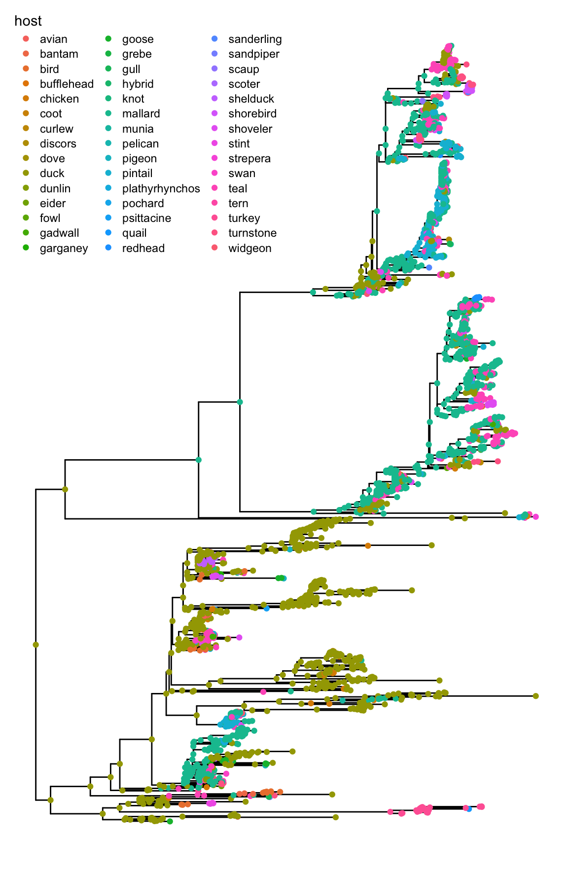
Figure 4.19: Example of integrating ggtree in analysis pipeline. A phylogenetic tree of H3 influenza viruses built by RAxML. Ancestral sequences were inferred by phangorn and ancestral host information estimated by ape. The ggtree allows integrating information for visualization and further analysis. The tree was annotated by symbolic circles colored by host information as in the legend at top right.
The ggtree can be integrated into analysis pipeline as demonstrated in this example and allows different diverse data sources to be combined into a tree object. As illustrated in this example, host information and ancestral sequences were stored in the tree object. Thereafter ggtree allows further comparison and analysis. For instance, users can associate amino acid substitution with host jump as demonstrated in Figure 4.20. Some sites (around position of 400) are conservative across different species and some sites (around position of 20) are frequently mutated especially for host jump to mallard (Figure 4.20A). Interestingly, mutations co-occurred with chicken-to-duck transmission tend to cluster in the HA global head; whereas the mutations distributed over the cytoplasmic tail of the HA are often leading to mallard transmission especially for teal-to-mallard and duck-to-mallard transmissions (Figure 4.20B). These results could direct the further experimental investigations of these markers, such as through reverse genetic studies.
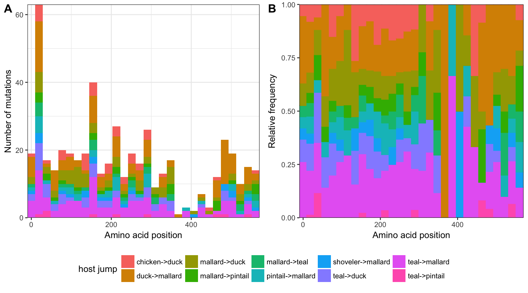
Figure 4.20: Amino acid substitution preferences. Different locations have different mutation frequencies. Mutations that lead to host jump have different preferences on mutation sites.
4.3.8 Performance comparison with other tree-related packages
Visualization and annotation of phylogenetic trees are possible thanks to many different packages. Especially in ape (Paradis, Claude, and Strimmer 2004) and phytools (Revell 2012), which provide many features of tree manipulation and visualization in base plotting system. The ggtree package brings various capabilities of phylogenetic visualization and annotation to the ggplot2 plotting system with high level of customizability possible thanks to the object-oriented approach of graphic and data communication. OutbreakTools (Jombart et al. 2014) and phyloseq (McMurdie and Holmes 2013) also implemented tree view functions using ggplot2 for presenting data from epidemiology and microbiome respectively. A comprehensive comparison of different features available in these packages can be found in Table ??. Here I present the benchmark performance of these packages. A random tree with 1000 leaves were used for basic tree visualization as shown in Figure 4.21. Basically ggtree and phyloseq are two most robust and fastest packages for viewing phylogenetic trees.
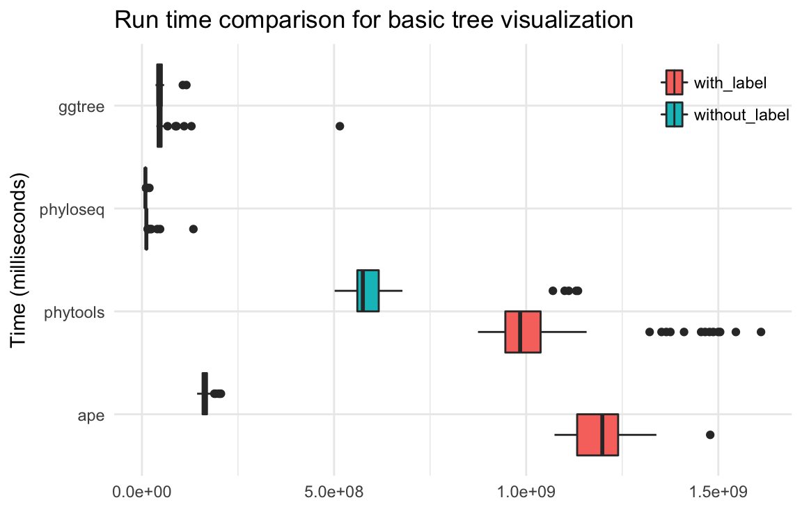
Figure 4.21: Run time comparison for basic tree visualization. Tree topology visualization with/without taxa name.
OutbreakTooks and phyloseq defined their own classes to store tree objects and specific data from epidemiology and microbiome respectively. OutbreakTools only works with obkData objects, while phyloseq works with phylo and phyloseq objects. As OutbreakTools cannot view phylo object, it was not incorporated in run time comparison of viewing phylogenetic trees. Although phyloseq can view phylo object, it lacks capability of annotating a phylogenetic tree with user data. To compare the performance of phylogenetic tree annotation, here I used ape and ggtree to reproduce examples presented in OutbreakTools and phyloseq vignettes. Noteably, S4 classes including obkData and phylose defined in OutbreakTools and phyloseq are also supported by ggtree and users can use + operator to add related annotation layers. As demonstrated in Figure 4.22, ape is the fastest package for tree annotation and ggtree outperform phyloseq and OutbreakTools.
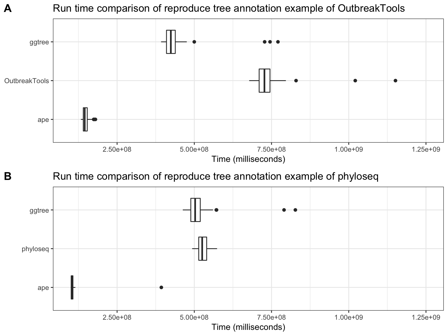
Figure 4.22: Run Time comparison for tree annotation. Reproducing tree annotation example of OutbreakTools and phyloseq using ape and ggtree.
To further compare visualizing phylogenetic trees with different numbers of leaves, here I used random trees with leaves ranging from 10 to 1000 with step by 10. As illustrated in Figure 4.23, ape and phytools are faster when trees are small while ggtree and phyloseq perform better with large tree.
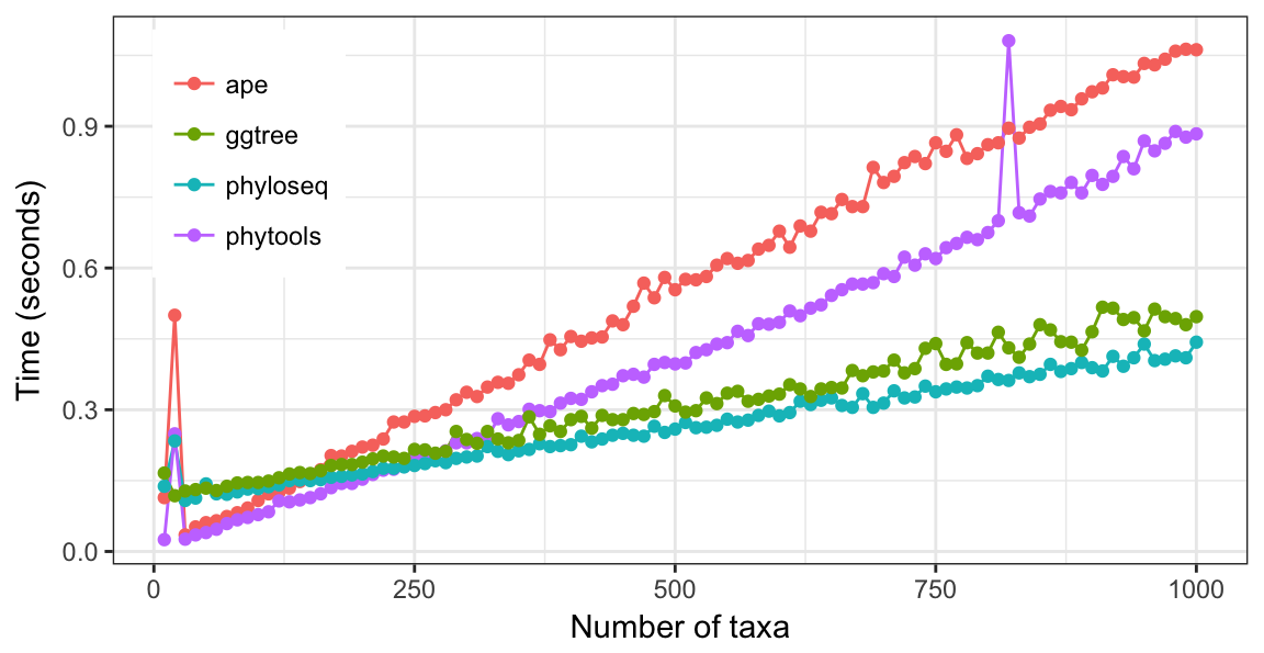
Figure 4.23: Run time of viewing tree with different numbers of leaves. The slowest time to view a phylogenetic tree with 1000 leaves is only 1 second. All these tools are fast enough for ordinary usages.
The benchmark was performed on iMac 3.2G Intel Core i5 with 16GB memory running OS X EI Capitan. Source code to reproduce benchmark results are presented in Figure ??, ??, ?? and ??. In the speed tests of ggtree and other packages using small to moderate size, ape and phytools are faster than ggtree and phyloseq. While for large tree, ggtree and phyloseq is faster than ape and phytools. For simple tree without annotation, phyloseq is faster than ggtree, while when annotating tree with multiple layers, ggtree is more efficient than both OutbreakTools and phyloseq. In addition, ggtree is a general tools that designed for tree annotation, while OutbreakTools and phyloseq are implemented for specific domain that lack of many features for general purpose of tree annotation. ggtree also provide grammar of graphic that are intuitive, easy to learn and allows high level of customization that are not available in other packages. In general, the performance of ggtree is more stable with different size of trees and different layers of annotation. The ggtree run fast in most of the tree visualization and annotation problems especially excels at large tree visualization and complex tree annotation.
4.4 Discussion
Creating a tree figure annotated with associated information (from experimental analyses, evolutionary inferences, etc.) is an important part of research on molecular evolution. Most of the tree viewing software lack the utilities to incorporate data from multiple external sources or by parsing files generated by other analysis programs/packages. FigTree is one of the commonly used software for tree visualization and annotation, whereas it mainly supports parsing BEAST output and not from other tools to annotate the tree. FigTree is a typical viewer in this field that designed for specific data type and implemented pre-defined annotation for specific needs.
Tools for visualizing phylogenetic trees are proliferating. Producing a publication-ready informative tree figure typically involves a series of annotation steps and requires several software packages to generate a static image as an end product. Such static image doesn’t contain choices of selecting features (e.g. ancestral state) that used to render the tree (e.g. as text label or branch width). This process is often one-way that has no route to return to previous annotation steps. It is often difficult to modify or reuse the underlying annotation information in other contexts (e.g., add a new layer of clade support value on the same tree). Therefore, repeated creations of similar complex tree figures for analysis or publication become extremely time-consuming.
Existing workflows are suboptimal from the standpoint of sharing and reuse. Tree visualization and annotation should contain a serialize compositions that preserve the selection and annotation in a portable format. This format can be modified (e.g., change color, add new layer etc.) and rendering the tree with annotation when needed. This way will make tree annotation more portable and transparent. The ggtree is designed to solve these issues. It can utilize evolutionary data from different tree objects (e.g., those parsed by treeio, see Chapter 2) as well as import other associated experimental data from external files, so that various sources and types of data can be displayed on a tree for comparison and further analyses. The ggtree also supports visualization of tree objects defined by other R packages so that ggtree can be easily integrated into existing analysis pipelines. For example, phyloseq tree object is supported by ggtree and microbiome data can be used to annotate the tree using ggtree.
The ggtree extends ggplot2 graphic system and allows creating separate geometric layers that can be freely combined, removed and rearranged to support diverse but convenient ways of tree manipulation and visualization. Layers defined in ggtree are not for specific purpose but serve as building blocks to annotate trees to meet users’ own needs in their favorite way.
The ggtree generates an image file of tree figures when users render the output object to an image file. Instead of producing an image file that can hardly be modified and reused, ggtree outputs a ggtree object that contains a serialized data that preserve the tree and associated data with layers of different data for tree tree annotation. These data (including tree, annotation data and layers) can be manipulated to modify tree, reuse data and adding/modifying layers of tree annotation.
The ggtree fits the ecosystem of R community as it supports most of the tree objects defined by the community and can be easily integrated to existing workflows. It also works with other packages to enhance its interoperability, for example, ggtree works with ggbio (Yin, Cook, and Lawrence 2012) package to visualize phylogenetic tree with genomic features and works with ggseqlogo10 package to annotate phylogenetic tree with sequence logo (Figure ??).
Using ggtree, large phylogenetic tree figures with complex annotations can be more easily and consistently generated. This is particular useful for those studying the virus genome and evolution. The recent rise of the field ‘phylodynamics’ has been widely applied in influenza research, and many studies in literature were trying to identify the association between the dynamic virus phenotypes and evolution (Loverdo and Lloyd-Smith 2013, Koelle et al. (2006)). Our ggtree could become an essential platform for high-level analysis of the data resulting from different types of evolutionary analyses.
References
Page, Roderic D. M. 2002. “Visualizing Phylogenetic Trees Using TreeView.” Current Protocols in Bioinformatics Chapter 6 (August): Unit 6.2. doi:10.1002/0471250953.bi0602s01.
Chevenet, François, Christine Brun, Anne-Laure Bañuls, Bernard Jacq, and Richard Christen. 2006. “TreeDyn: Towards Dynamic Graphics and Annotations for Analyses of Trees.” BMC Bioinformatics 7 (October): 439. doi:10.1186/1471-2105-7-439.
Huson, Daniel H., and Celine Scornavacca. 2012. “Dendroscope 3: An Interactive Tool for Rooted Phylogenetic Trees and Networks.” Systematic Biology 61 (6): 1061–7. doi:10.1093/sysbio/sys062.
He, Zilong, Huangkai Zhang, Shenghan Gao, Martin J. Lercher, Wei-Hua Chen, and Songnian Hu. 2016. “Evolview V2: An Online Visualization and Management Tool for Customized and Annotated Phylogenetic Trees.” Nucleic Acids Research 44 (W1): W236–241. doi:10.1093/nar/gkw370.
Letunic, Ivica, and Peer Bork. 2007. “Interactive Tree of Life (iTOL): An Online Tool for Phylogenetic Tree Display and Annotation.” Bioinformatics 23 (1): 127–28. doi:10.1093/bioinformatics/btl529.
R Core Team. 2016. R: A Language and Environment for Statistical Computing. Vienna, Austria: R Foundation for Statistical Computing. https://www.R-project.org/.
Gentleman, Robert C, Vincent J Carey, Douglas M Bates, Ben Bolstad, Marcel Dettling, Sandrine Dudoit, Byron Ellis, et al. 2004. “Bioconductor: Open Software Development for Computational Biology and Bioinformatics.” Genome Biology 5 (10): R80. doi:10.1186/gb-2004-5-10-r80.
Wickham, Hadley. 2016. Ggplot2: Elegant Graphics for Data Analysis. Springer. http://ggplot2.org.
Wilkinson, Leland, D. Wills, D. Rope, A. Norton, and R. Dubbs. 2005. The Grammar of Graphics. 2nd edition. New York: Springer.
Paradis, Emmanuel, Julien Claude, and Korbinian Strimmer. 2004. “APE: Analyses of Phylogenetics and Evolution in R Language.” Bioinformatics 20 (2): 289–90. doi:10.1093/bioinformatics/btg412.
Revell, Liam J. 2012. “Phytools: An R Package for Phylogenetic Comparative Biology (and Other Things).” Methods in Ecology and Evolution 3 (2): 217–23. doi:10.1111/j.2041-210X.2011.00169.x.
Jombart, Thibaut, David M. Aanensen, Marc Baguelin, Paul Birrell, Simon Cauchemez, Anton Camacho, Caroline Colijn, et al. 2014. “OutbreakTools: A New Platform for Disease Outbreak Analysis Using the R Software.” Epidemics 7 (June): 28–34. doi:10.1016/j.epidem.2014.04.003.
McMurdie, Paul J., and Susan Holmes. 2013. “Phyloseq: An R Package for Reproducible Interactive Analysis and Graphics of Microbiome Census Data.” PloS One 8 (4): e61217. doi:10.1371/journal.pone.0061217.
Lam, Tommy Tsan-Yuk, Chung-Chau Hon, Philippe Lemey, Oliver G. Pybus, Mang Shi, Hein Min Tun, Jun Li, Jingwei Jiang, Edward C. Holmes, and Frederick Chi-Ching Leung. 2012. “Phylodynamics of H5N1 Avian Influenza Virus in Indonesia.” Molecular Ecology 21 (12): 3062–77. doi:10.1111/j.1365-294X.2012.05577.x.
Retief, J. D. 2000. “Phylogenetic Analysis Using PHYLIP.” Methods in Molecular Biology (Clifton, N.J.) 132: 243–58.
Wilgenbusch, James C., and David Swofford. 2003. “Inferring Evolutionary Trees with PAUP*.” Current Protocols in Bioinformatics Chapter 6 (February): Unit 6.4. doi:10.1002/0471250953.bi0604s00.
Neher, Richard A., Trevor Bedford, Rodney S. Daniels, Colin A. Russell, and Boris I. Shraiman. 2016. “Prediction, Dynamics, and Visualization of Antigenic Phenotypes of Seasonal Influenza Viruses.” Proceedings of the National Academy of Sciences 113 (12): E1701–E1709. doi:10.1073/pnas.1525578113.
Liang, Huyi, Tommy Tsan-Yuk Lam, Xiaohui Fan, Xinchun Chen, Yu Zeng, Ji Zhou, Lian Duan, et al. 2014. “Expansion of Genotypic Diversity and Establishment of 2009 H1N1 Pandemic-Origin Internal Genes in Pigs in China.” Journal of Virology, July, JVI.01327–14. doi:10.1128/JVI.01327-14.
Kuczynski, Justin, Jesse Stombaugh, William Anton Walters, Antonio González, J. Gregory Caporaso, and Rob Knight. 2011. “Using QIIME to Analyze 16S rRNA Gene Sequences from Microbial Communities.” Current Protocols in Bioinformatics / Editoral Board, Andreas D. Baxevanis ... [et Al.] CHAPTER (December): Unit10.7. doi:10.1002/0471250953.bi1007s36.
Schloss, Patrick D., Sarah L. Westcott, Thomas Ryabin, Justine R. Hall, Martin Hartmann, Emily B. Hollister, Ryan A. Lesniewski, et al. 2009. “Introducing Mothur: Open-Source, Platform-Independent, Community-Supported Software for Describing and Comparing Microbial Communities.” Applied and Environmental Microbiology 75 (23): 7537–41. doi:10.1128/AEM.01541-09.
Callahan, Benjamin J., Paul J. McMurdie, Michael J. Rosen, Andrew W. Han, Amy Jo A. Johnson, and Susan P. Holmes. 2016. “DADA2: High-Resolution Sample Inference from Illumina Amplicon Data.” Nature Methods 13 (7): 581–83. doi:10.1038/nmeth.3869.
Kunin, Victor, and Philip Hugenholtz. 2010. “PyroTagger : A Fast , Accurate Pipeline for Analysis of rRNA Amplicon Pyrosequence Data.” The Open Journal, 1–8. http://www.theopenjournal.org/toj_articles/1.
Edgar, Robert C. 2004. “MUSCLE: Multiple Sequence Alignment with High Accuracy and High Throughput.” Nucleic Acids Research 32 (5): 1792–7. doi:10.1093/nar/gkh340.
Stamatakis, Alexandros. 2014. “RAxML Version 8: A Tool for Phylogenetic Analysis and Post-Analysis of Large Phylogenies.” Bioinformatics 30 (9): 1312–3. doi:10.1093/bioinformatics/btu033.
Schliep, Klaus Peter. 2011. “Phangorn: Phylogenetic Analysis in R.” Bioinformatics 27 (4): 592–93. doi:10.1093/bioinformatics/btq706.
Yin, Tengfei, Dianne Cook, and Michael Lawrence. 2012. “Ggbio: An R Package for Extending the Grammar of Graphics for Genomic Data.” Genome Biology 13 (8): R77. doi:10.1186/gb-2012-13-8-r77.
Loverdo, Claude, and James O. Lloyd-Smith. 2013. “INTER-GENERATIONAL PHENOTYPIC MIXING IN VIRAL EVOLUTION.” Evolution; International Journal of Organic Evolution 67 (6): 1815–22. doi:10.1111/evo.12048.
Koelle, Katia, Sarah Cobey, Bryan Grenfell, and Mercedes Pascual. 2006. “Epochal Evolution Shapes the Phylodynamics of Interpandemic Influenza A (H3N2) in Humans.” Science (New York, N.Y.) 314 (5807): 1898–1903. doi:10.1126/science.1132745.