ggupset -- ggplot2版本的upset plot
在《一图告诉你venn plot和upset plot的关系》一文中,我们应该很清楚这两者的关系,upset plot是更清晰的呈现方式,而且能够支持无数多个分类,在《转UpSet图为ggplot?》一文中,又介绍了一个转化UpSetR输出为ggplot2便于嵌图和拼图的方法,但这个需要一个补丁,然后我提交的这个补丁,一直没有被作者接收。而且毕竟UpSetR是用grid写的,像grid这种高级货,玩起来还是有点难度,我一直在想应该有一个ggplot2版本的upset plot,最近就让我在gayhub上发现了。
这包已经在CRAN上,所以可以用最简单的方式安装:
install.packages("ggupset")
library(tidyverse)
library(ggupset)
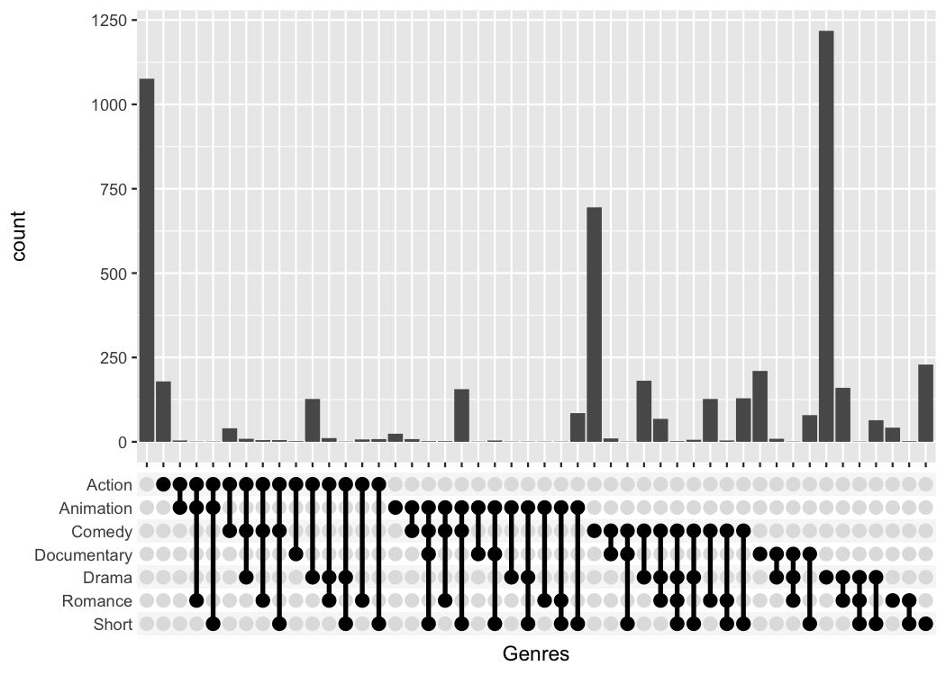
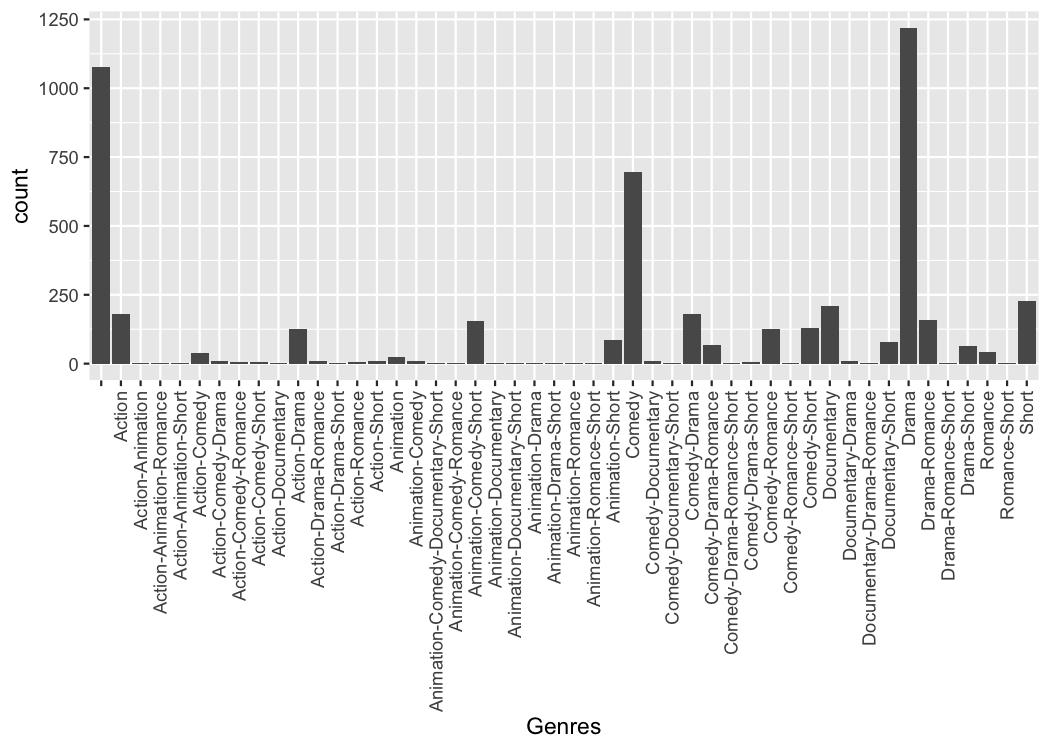
tidy_movies %>%
distinct(title, year, length, .keep_all=TRUE) %>%
ggplot(aes(x=Genres)) +
geom_bar() +
scale_x_upset(n_intersections = 20)
它的做法是把x-axis给改了,不过我发现还有一个不太兼容的地方,你不能对输出使用theme,像上面的图,你如果+theme_bw()就会报错。但好在你可以在scale_x_upset前面加theme,也还OK。
比如你想应用theme_bw,则必须是:
tidy_movies %>%
  distinct(title, year, length, .keep_all=TRUE) %>%
  ggplot(aes(x=Genres)) +
    geom_bar() +
    theme_bw() + #加在最后则不行
    scale_x_upset(n_intersections = 20)
这样等同于说下面那部分,你没法用theme去控制,所以作者又提供了theme_combmatrix来控制下面那部分。
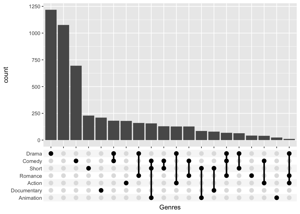
tidy_movies %>%
  distinct(title, year, length, .keep_all=TRUE) %>%
  ggplot(aes(x=Genres)) +
    geom_bar() +
    scale_x_upset(order_by = "degree") +
    theme_combmatrix(combmatrix.panel.point.color.fill = "green",
                     combmatrix.panel.line.size = 0,
                     combmatrix.label.make_space = FALSE)
用ggplot2的好处
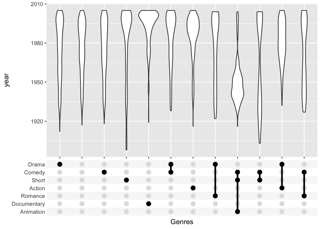
用grid就是封装,ggplot2虽然是基于grid,但为什么大家这么爱ggplot2,因为它的设计是抽象,所有的东西是乐高块,我们可以自己拼,像上面所提到的,ggupset实现的是另一种x-axis,那么各种x轴是分类型变量的图,就可以应用这样的x坐标,于是有了自由的选项,高级的图应运而生。
tidy_movies %>%
  distinct(title, year, length, .keep_all=TRUE) %>%
  ggplot(aes(x=Genres, y=year)) +
    geom_violin() +
    scale_x_upset(order_by = "freq", n_intersections = 12)
df_complex_conditions %>%
  mutate(Label = pmap(list(KO, DrugA, Timepoint), function(KO, DrugA, Timepoint){
    c(if(KO) "KO" else "WT", if(DrugA == "Yes") "Drug", paste0(Timepoint, "h"))
  })) %>%
  ggplot(aes(x=Label, y=response)) +
    geom_boxplot() +
    geom_jitter(aes(color=KO), width=0.1) +
    geom_smooth(method = "lm", aes(group = paste0(KO, "-", DrugA))) +
    scale_x_upset(order_by = "degree",
                  sets = c("KO", "WT", "Drug", "8h", "24h", "48h"),
                  position="top", name = "") +
    theme_combmatrix(combmatrix.label.text = element_text(size=12),
                     combmatrix.label.extra_spacing = 5)
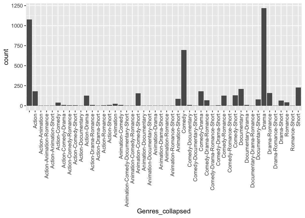
tidy_movies %>%
  mutate(Genres_collapsed = sapply(Genres, function(x) paste0(sort(x), collapse="-"))) %>%
  mutate(Genres_collapsed = fct_lump(fct_infreq(as.factor(Genres_collapsed)), n=12)) %>%
  group_by(stars, Genres_collapsed) %>%
  summarize(percent_rating = sum(votes * percent_rating)) %>%
  group_by(Genres_collapsed) %>%
  mutate(percent_rating = percent_rating / sum(percent_rating)) %>%
  arrange(Genres_collapsed) %>%
  ggplot(aes(x=Genres_collapsed, y=stars, fill=percent_rating)) +
    geom_tile() +
    stat_summary_bin(aes(y=percent_rating * stars), fun.y = sum,  geom="point",
                     shape="—", color="red", size=6) +
    axis_combmatrix(sep = "-", levels = c("Drama", "Comedy", "Short",
                    "Documentary", "Action", "Romance", "Animation", "Other")) +
    scale_fill_viridis_c()