Phylogenetic Tree Annotation
This lesson introduces basic annotation utilies for common tasks such as highlight and labelling clades.
Label Clade
library(ggtree)
set.seed(2015-12-21)
tree <- rtree(30)
p <- ggtree(tree) + xlim(NA, 6)

p + geom_cladelabel(node=45, label="test label") +
    geom_cladelabel(node=34, label="another clade")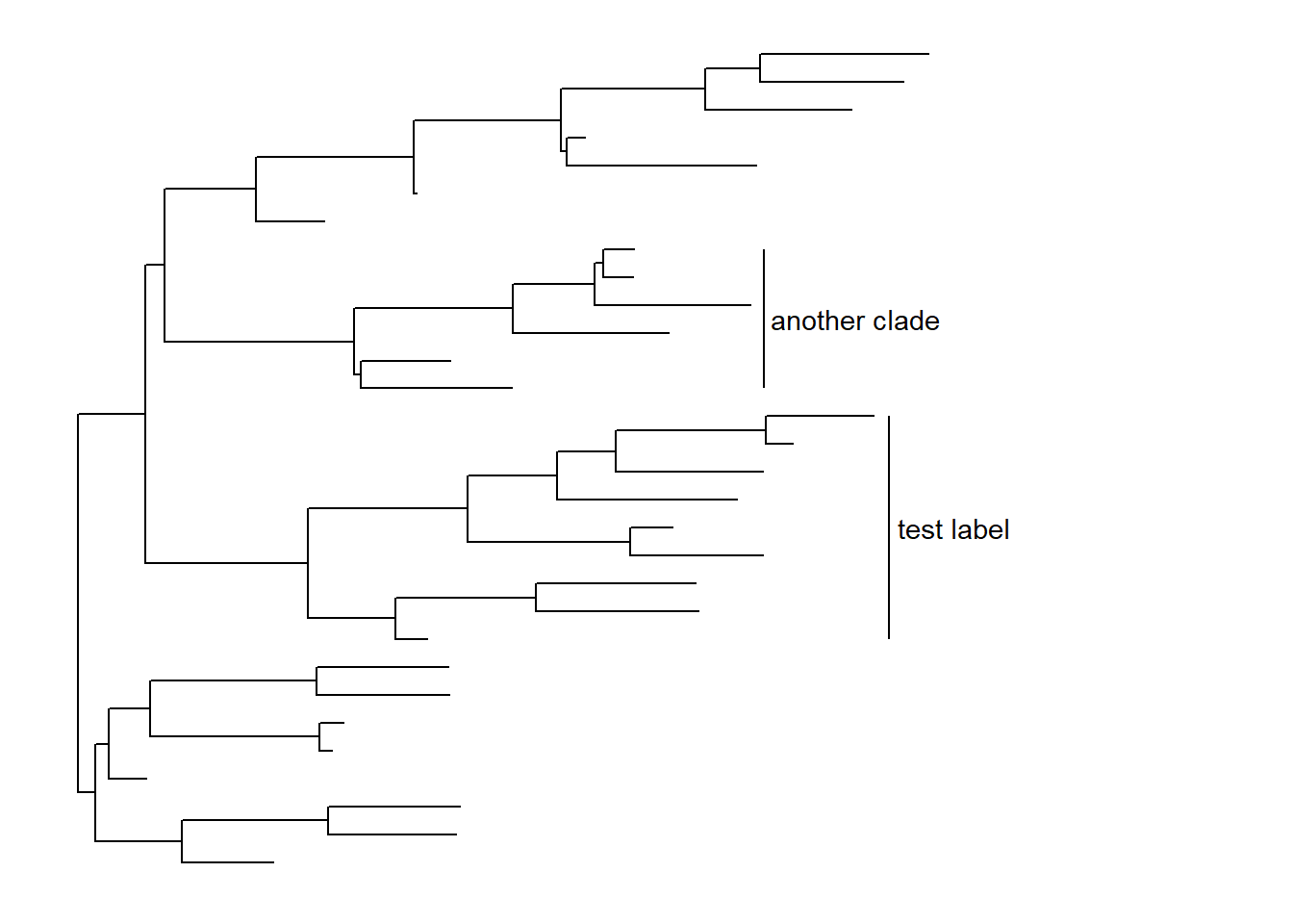
We can use align=TRUE to align the clade label and use offset to adjust the position.
p + geom_cladelabel(node=45, label="test label", align=T, color='red') +
    geom_cladelabel(node=34, label="another clade", align=T, color='blue')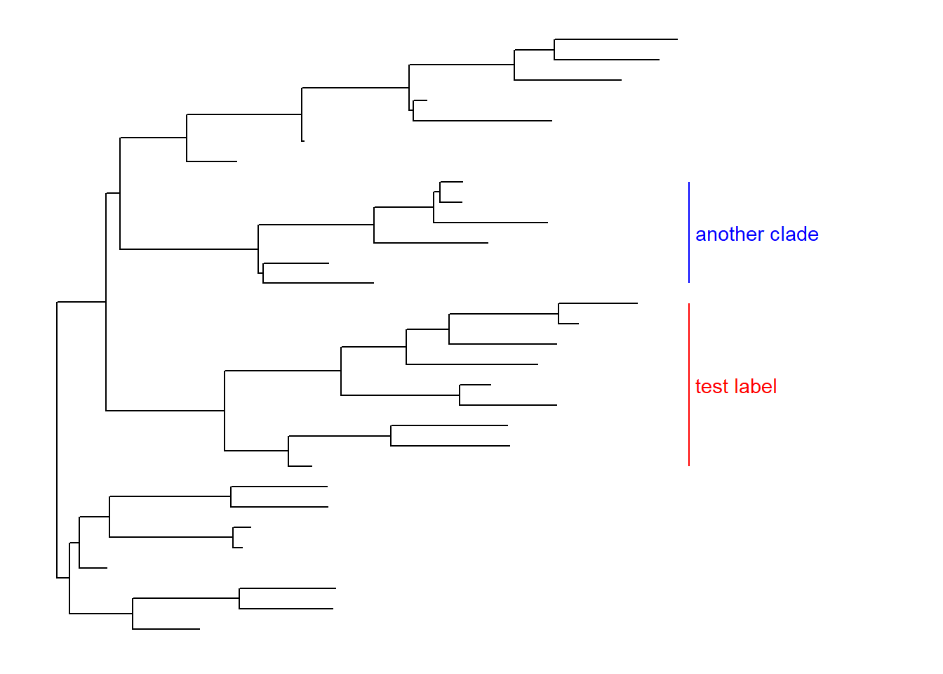
Exercise 1
Look at the help for ?geom_cladelabel to learn the usages of other parameters.
- rotate the text ’another clade` with 45 degree.
- increase the sizes of bar and label for the ‘test label’
- increase relative positon of bar and label
Highlight clades
ggtree implements geom_hilight to add rectangle to highlight selected clade.
ggtree(tree) + geom_hilight(node=34, fill="steelblue", alpha=.6) +
    geom_hilight(node=45, fill="darkgreen", alpha=.6)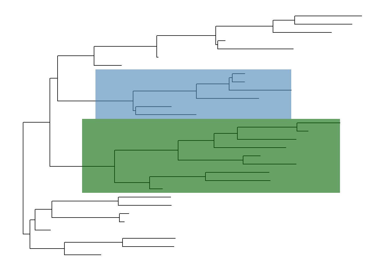
geom_hilight supports rectangular and circular layouts. For unrooted layout, ggtree provides geom_hilight_encircle layer.
ggtree(tree, layout = "unrooted") + geom_hilight_encircle(node=34, fill='steelblue') +
  geom_hilight_encircle(node=45, fill="darkgreen")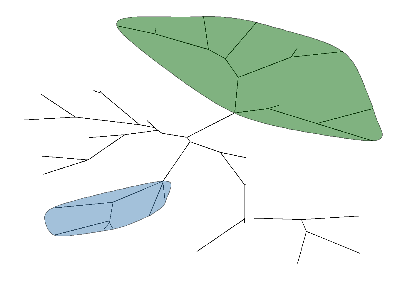
Exercise 2
- Create a circular layout tree and highlight the selected clades.
Uncertainty of evolutionary inference
ggtree provides geom_range to display uncertainty of evolutionary inference.
This example use a BEAST tree, which was imported by treeio. Data that stored in the tree object or mapped to the tree from external data can be used to annotate the tree directly.
beast_tree <- read.beast("data/MCC_FluA_H3.tree")
ggtree(beast_tree) + geom_range(range = 'height_0.95_HPD', branch.length='height', color='red', alpha=.6, size=2)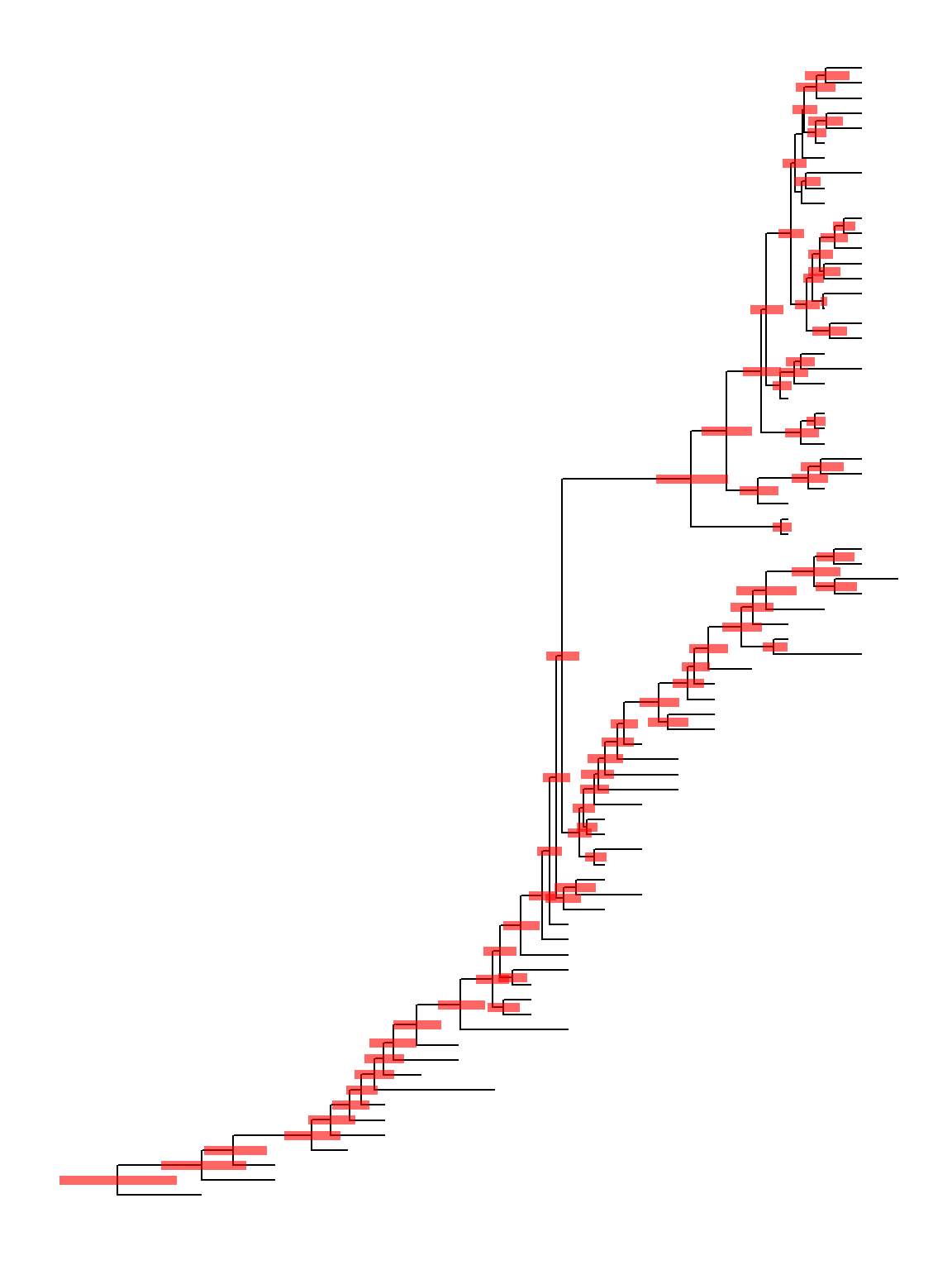
Exercise 3
- create a heat tree by using substitution rate (
rateinbeast_tree) to color branches.
Visualize tree with associated matrix (as a heatmap)
Visualizing tree with external data will mainly be introduced in next lesson. As visualizing heatmap and multiple sequence alignment with the tree are frequently used, ggtree provides gheatmap and msaplot function for these tasks.
genotype <- read.table("data/Genotype.txt", sep="\t", stringsAsFactor=F)
colnames(genotype) <- sub("\\.$", "", colnames(genotype))
p <- ggtree(beast_tree) + geom_tiplab(size=2)
gheatmap(p, genotype, offset=8, width=0.6, font.size=3) +
  scale_fill_brewer(palette="Set2", breaks=c("HuH3N2", "pdm", "trig"))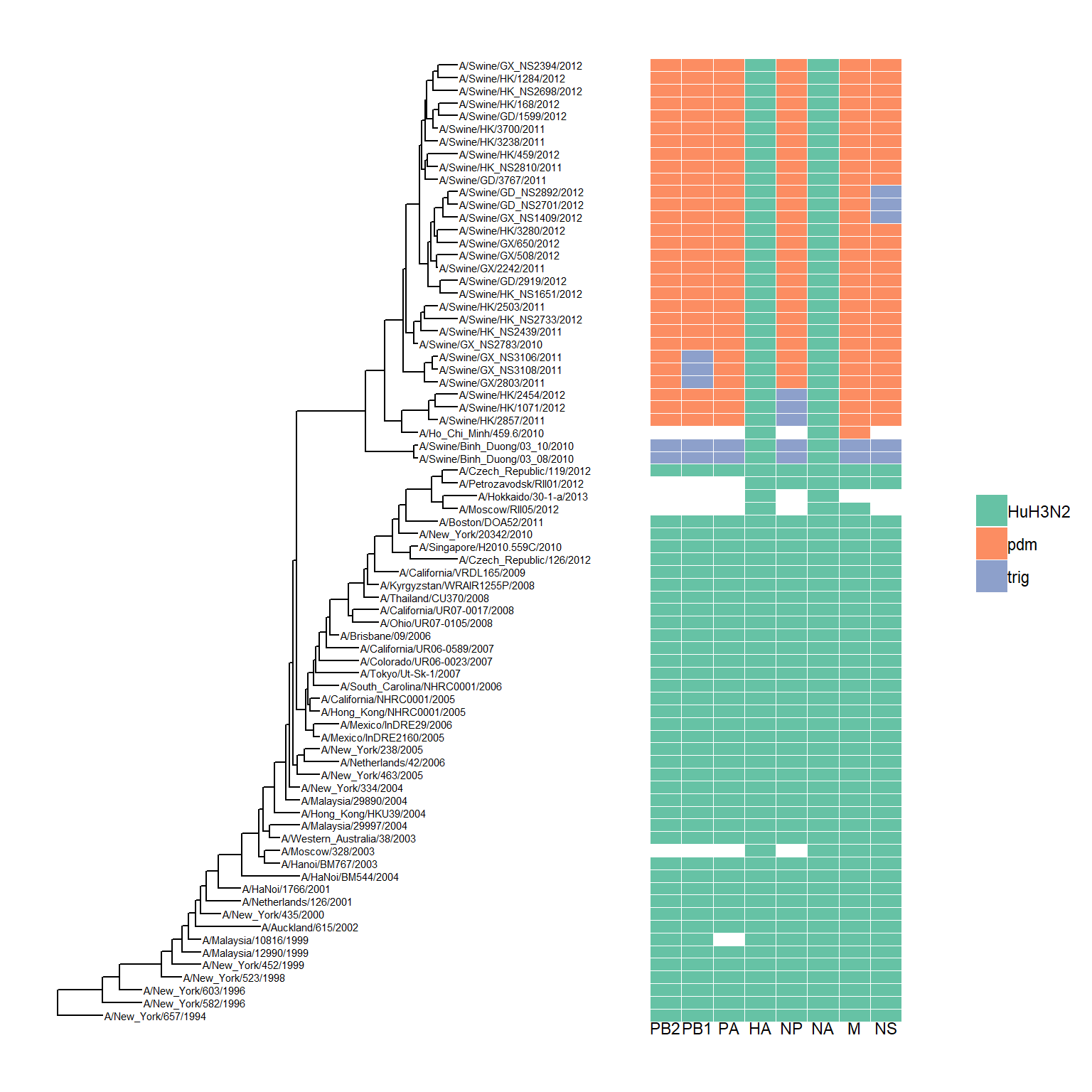
Exercise 4
- Read the Cookbook for R and re-create this figure with another color palette, e.g.
Paired. - create a tree with heatmap in circular layout
Visualize tree with multiple sequence alignment
The msaplot accepts a tree (output of ggtree) and a fasta file, then it can visualize the tree with sequence alignment. We can specify the width (relative to the tree) of the alignment and adjust relative position by offset, that are similar to gheatmap function.
tree <- read.tree("data/tree.nwk")
p <- ggtree(tree) + geom_tiplab(size=3)
msaplot(p, "data/sequence.fasta", offset=3, width=2)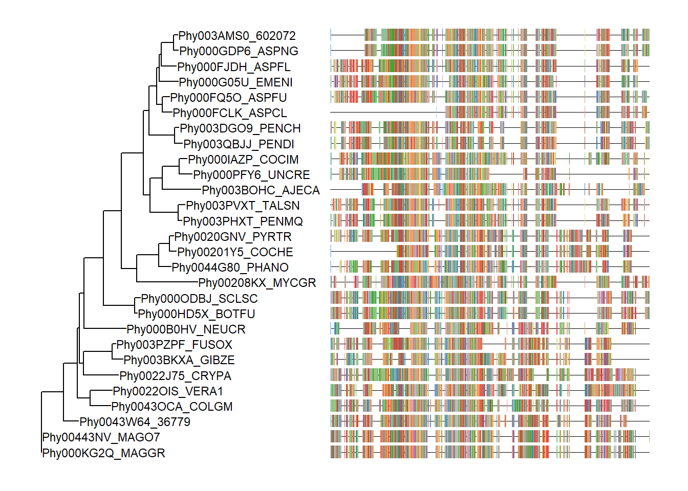
Exercise 5
- plot tree with MSA at specific slide of the alignment (e.g. at the position of [300, 350])
- re-create the above figure using circular layout