one-dimensional integrals

The foundamental idea of numerical integration is to estimate the area of the region in the xy-plane bounded by the graph of function f(x). The integral was esimated by dividing x into small intervals, then adds all the small approximations to give a total approximation.

Trapezoidal rule

Numerical integration can be done by trapezoidal rule, simpson’s rule and quadrature rules. R has a built-in function, integrate, which performs adaptive quadrature.

Trapezoidal rule works by approximating the region under the graph f(x) as a trapezoid and calculating its area.

trapezoid <- function(fun, a, b, n=100) {
    # numerical integral of fun from a to b
    # using the trapezoid rule with n subdivisions
    # assume a < b and n is a positive integer
    h <- (b-a)/n
    x <- seq(a, b, by=h)
    y <- fun(x)
    s <- h * (y[1]/2 + sum(y[2:n]) + y[n+1]/2)
    return(s)
}

Simpson’s rule

Simpson’s rule subdivides the interval [a,b] into n subintervals, where n is even, then on each consecutive pairs of subintervals, it approximates the behaviour of f(x) by a parabola (polynomial of degree 2) rather than by the straight lines used in the trapezoidal rule.

simpson <- function(fun, a, b, n=100) {
    # numerical integral using Simpson's rule
    # assume a < b and n is an even positive integer
    h <- (b-a)/n
    x <- seq(a, b, by=h)
    if (n == 2) {
        s <- fun(x[1]) + 4*fun(x[2]) +fun(x[3])
    } else {
        s <- fun(x[1]) + fun(x[n+1]) +
        	2*sum(fun(x[seq(2,n,by=2)])) + 
            4 *sum(fun(x[seq(3,n-1, by=2)]))
    }
    s <- s*h/3
    return(s)
}

To calculate an integrate over infinite interval, one way is to transform it into an integral over a finite interval as introduce in wiki.

simpson_v2 <- function(fun, a, b, n=100) {
    # numerical integral using Simpson's rule
    # assume a < b and n is an even positive integer
    if (a == -Inf & b == Inf) {
        f <- function(t) (fun((1-t)/t) + fun((t-1)/t))/t^2
        s <- simpson_v2(f, 0, 1, n)
    } else if (a == -Inf & b != Inf) {
        f <- function(t) fun(b-(1-t)/t)/t^2
        s <- simpson_v2(f, 0, 1, n)
    } else if (a != -Inf & b == Inf) {
        f <- function(t) fun(a+(1-t)/t)/t^2
        s <- simpson_v2(f, 0, 1, n)
    } else {
        h <- (b-a)/n
        x <- seq(a, b, by=h)
        y <- fun(x)
        y[is.nan(y)]=0
        s <- y[1] + y[n+1] + 
        	2*sum(y[seq(2,n,by=2)]) + 
            4 *sum(y[seq(3,n-1, by=2)])
        s <- s*h/3
    }
    return(s)
}

> phi <- function(x) exp(-x^2/2)/sqrt(2*pi)  ##normal distribution
> simpson_v2(phi, 0, Inf, n=100)
[1] 0.4986569
> simpson_v2(phi, -Inf,3, n=100)
[1] 0.998635
> pnorm(3)
[1] 0.9986501

Simpson’s rule is more accuracy than trapezoidal rule. To compare the accuracy between simpson’s rule and trapezoidal rule, I estimated $ \int_{0.01}^{1} \frac{1}{x} dx = -\log(0.01)$ for a sequence of increasing values of n.

f <- function(x) 1/x
#integrate(f, 0.01, 1) == -log(0.01)
S.trapezoid <- function(n) trapezoid(f, 0.01, 1, n)
S.simpson <- function(n) simpson(f, 0.01, 1, n)

n <- seq(10, 1000, by = 10)
St <- sapply(n, S.trapezoid)
Ss <- sapply(n, S.simpson)

opar <- par(mfrow = c(2, 2))
plot(n,St + log(0.01), type="l", xlab="n", ylab="error", main="Trapezoidal rule")
plot(n,Ss + log(0.01), type="l", xlab="n", ylab="error",main="Simpson's rule")
plot(log(n), log(St+log(0.01)),type="l", xlab="log(n)", ylab="log(error)",main="Trapezoidal rule")
plot(log(n), log(Ss+log(0.01)),type="l", xlab="log(n)", ylab="log(error)",main="Simpson's rule")

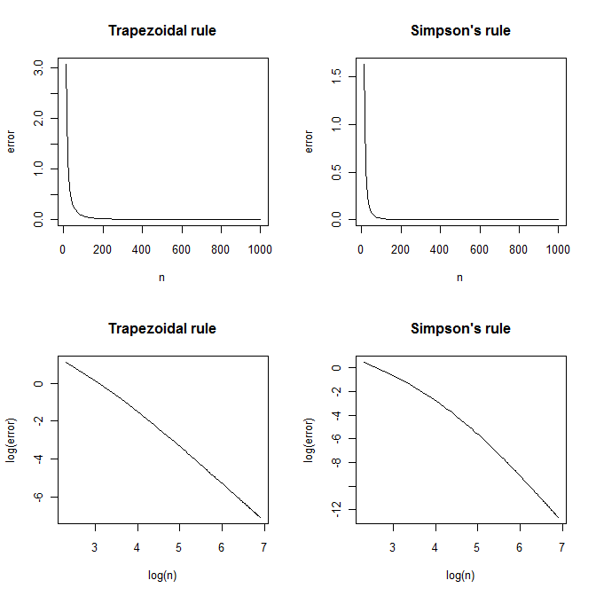
The plot showed that log(error) against log(n) appears to have a slope of -1.90 and -3.28 for trapezoidal rule and simpson’s rule respectively.

Another way to compare their accuracy is to calculate how large of the partition size n for reaching a specific tolerance.

yIntegrate <- function(fun, a, b, tol=1e-8, method= "simpson", verbose=TRUE) {
    # numerical integral of fun from a to b, assume a < b 
    # with tolerance tol
    n <- 4
    h <- (b-a)/4
    x <- seq(a, b, by=h)
    y <- fun(x)
    yIntegrate_internal <- function(y, h, n, method) {
        if (method == "simpson") {
            s <- y[1] + y[n+1] + 4*sum(y[seq(2,n,by=2)]) + 
            	2 *sum(y[seq(3,n-1, by=2)])
            s <- s*h/3
        } else if (method == "trapezoidal") {
            s <- h * (y[1]/2 + sum(y[2:n]) + y[n+1]/2)
        } else {
        }       
        return(s)
    }
    
    s <- yIntegrate_internal(y, h, n, method)
    s.diff <- tol + 1 # ensures to loop at once.
    while (s.diff > tol ) {
        s.old <- s
        n <- 2*n
        h <- h/2
        y[seq(1, n+1, by=2)] <- y ##reuse old fun values
        y[seq(2,n, by=2)] <- sapply(seq(a+h, b-h, by=2*h), fun)
        s <- yIntegrate_internal(y, h, n, method)
        s.diff <- abs(s-s.old)
    }
    if (verbose) {
        cat("partition size", n, "\n")
    }
    return(s)
}

> fun <- function(x) exp(x) - x^2
> yIntegrate(fun, 3,5,tol=1e-8, method="simpson")
partition size 512 
[1] 95.66096
> yIntegrate(fun, 3,5,tol=1e-8, method="trapezoidal")
partition size 131072 
[1] 95.66096

As show above, simpson’s rule converge much faster than trapezoidal rule.

Quadrature rule

Quadrature rule is more efficient than traditional algorithms. In adaptive quadrature, the subinterval width h is not constant over the interval [a,b], but instead adapts to the function. Here, I presented the adaptive simpson’s method.

quadrature <- function(fun, a, b, tol=1e-8) {
    # numerical integration using adaptive quadrature
    
    quadrature_internal <- function(S.old, fun, a, m, b, tol, level) {
        level.max <- 100
        if (level > level.max) {
            cat ("recursion limit reached: singularity likely\n")
            return (NULL)
        }
        S.left <- simpson(fun, a, m, n=2) 
        S.right <- simpson(fun, m, b, n=2)
        S.new <- S.left + S.right
        if (abs(S.new-S.old) > tol) {
            S.left <- quadrature_internal(S.left, fun, a, (a+m)/2, m, tol/2, level+1)
            S.right <- quadrature_internal(S.right, fun, m, (m+b)/2, b, tol/2, level+1)
            S.new <- S.left + S.right
        }
        return(S.new)
    }
    
    level = 1
    S.old <- (b-a) * (fun(a) + fun(b))/2
    S.new <- quadrature_internal(S.old, fun, a, (a+b)/2, b, tol, level+1)
    return(S.new)
}

Quadrature rule is effective when f(x) is steep.

> fun <- function(x) return(1.5 * sqrt(x))
> system.time(yIntegrate(fun, 0,1, tol=1e-9, method="simpson"))
partition size 524288 
   user  system elapsed 
   1.58    0.00    1.58 
> system.time(quadrature(fun, 0,1, tol=1e-9))
   user  system elapsed 
   0.25    0.00    0.25

Reference

Robinson A., O. Jones, and R. Maillardet. 2009. Introduction to Scientific Programming and Simulation Using R. Chapman and Hall.
http://en.wikipedia.org/wiki/Numerical_integration
http://en.wikipedia.org/wiki/Trapezoidal_rule
http://en.wikipedia.org/wiki/Simpson%27s_rule
http://en.wikipedia.org/wiki/Adaptive_quadrature

one-dimensional integrals

Trapezoidal rule

Simpson’s rule

Quadrature rule

Reference

Guangchuang Yu